Overview
I recently had the great pleasure to meet with Professor Allan Just and he introduced me to eXtreme Gradient Boosting (XGBoost). I have extended the earlier work on my old blog by comparing the results across XGBoost, Gradient Boosting (GBM), Random Forest, Lasso, and Best Subset. The ensemble method is powerful as it combines the predictions from multiple machine learning algorithms together to make more accurate predictions than an individual model. Random Forest is among the most famous ones and it is easy to use. Random Forest is based on bagging (bootstrap aggregation) which averages the results over many decision trees from sub-samples. It further limits its search to only 1/3 of the features (in regression) to fit each tree, weakening the correlations among decision trees. It is easy to get a lower testing error compared to linear models.
Boosting takes slower steps, making predictors sequentially instead of independently. It repetitively leverages the patterns in residuals, strengthens the model with weak predictions, and make it better. By combining the advantages from both random forest and gradient boosting, XGBoost gave the a prediction error ten times lower than boosting or random forest in my case.
(Correction!) 18.10.3. When I further test this dataset I realized it was a mistake. There is indeed no magic in machine learning. When I got a testing error ten-time smaller than other methods, I should question first if this is a mistake. In the correct result XGBoost still gave the lowest testing rmse but was close to other two methods.
Link to the earlier version: Model Selection using Lasso and Best Subset
About the Data
In sub-Saharan Africa, the region where deprivations in terms of living conditions are the most severe, slum dwellers represent an estimated 56% of the regions’ urban population (UN Habitat, 2016). Measuring informal settlements in a reliable way is a critical challenge for the United Nations to monitor the Sustainable Development Goals (SDGs) towards its 2030 Agenda for Sustainable Development. This data was collected by Slum Dwellers International (SDI), which was nominated for the Nobel Peace Prize in 2014. By extracting valuable information from the data, We will help the UN to create better SDG indicators by making full use of available data.
In this exercise, we only model Share_Temporary: Share of Temporary Structure in Slums as the dependent variable. The independent variables are monitoring indicators like water, sanitation, housing conditions and overcrowding in African slum settlements. Dataset dimension is 973 x 153.
1. Extreme Gradient Boosting
- Random search: randomized parameters and update the record with best ones.
- It turns out to be a very interesting method to scan for hyperparameters. It will take a while for 100 iters.
- The package
xgboostis really fast.
library(xgboost)
# Randomize and bound
best_param <- list()
best_seednumber <- 1234
best_rmse <- Inf
best_rmse_index <- 0

set.seed(1234)
# In reality, might need 100 or 200 iters
for (iter in 1:10) {
  param <- list(objective = "reg:linear",  # For regression
                eval_metric = "rmse",      # rmse is used for regression
                max_depth = sample(6:10, 1),
                eta = runif(1, .01, .1),   # Learning rate, default: 0.3
                subsample = runif(1, .6, .9),
                colsample_bytree = runif(1, .5, .8),
                min_child_weight = sample(5:10, 1), # These two are important
                max_delta_step = sample(5:10, 1)    # Can help to focus error
                                                    # into a small range.
  )
  cv.nround <-  1000
  cv.nfold <-  5 # 5-fold cross-validation
  seed.number  <-  sample.int(10000, 1) # set seed for the cv
  set.seed(seed.number)
  mdcv <- xgb.cv(data = dtrain, params = param,
                 nfold = cv.nfold, nrounds = cv.nround,
                 verbose = F, early_stopping_rounds = 8, maximize = FALSE)

  min_rmse_index  <-  mdcv$best_iteration
  min_rmse <-  mdcv$evaluation_log[min_rmse_index]$test_rmse_mean

  if (min_rmse < best_rmse) {
    best_rmse <- min_rmse
    best_rmse_index <- min_rmse_index
    best_seednumber <- seed.number
    best_param <- param
  }
}- The best tuning parameters
##    objective eval_metric max_depth     eta subsample colsample_bytree
## 1 reg:linear        rmse         9 0.09822      0.64           0.6853
##   min_child_weight max_delta_step best_rmse_index best_rmse best_seednumber
## 1 6 8 56 0.2102 3660- MSE
## [22:09:43] WARNING: amalgamation/../src/objective/regression_obj.cu:174: reg:linear is now deprecated in favor of reg:squarederror.## [1] 0.04237- Feature Importance
importance_matrix <- xgb.importance(colnames(X_train), model = xg_mod)
# Use `xgb.plot.importance`, which create a _barplot_ or use `xgb.ggplot.importance`
library(Ckmeans.1d.dp) # for xgb.ggplot.importance
xgb.ggplot.importance(importance_matrix, top_n = 15, measure = "Gain")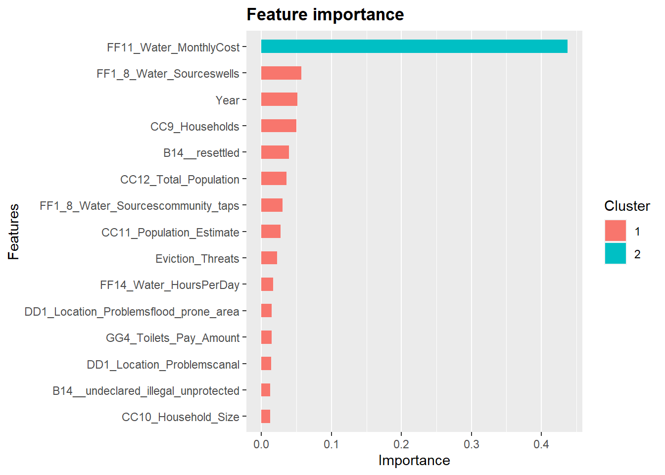
- Plot only 2 trees as an example (use
trees= 1)
library("DiagrammeR")
xgb.plot.tree(model = xg_mod, trees = 1, feature_names = colnames(X_train))- Plot all trees on one tree and plot it: A huge plot
xgb.plot.multi.trees(model = xg_mod, n_first_tree = 1, feature_names = colnames(X_train))2. Gradient boosting
- Use library
gbm
- Tuning Method: use
trainfunction fromcaretto scan a grid of parameters.
library(gbm)   # for Gradient boosting
library(caret) # scan the parameter grid using `train` function
# time_now <- Sys.time()
para_grid <- expand.grid(n.trees = (20*c(50:100)),
shrinkage = c(0.1, 0.05, 0.01),
interaction.depth = c(1,3,5),
n.minobsinnode = 10)
trainControl <- trainControl(method = "cv", number = 10)
set.seed(123)
gbm_caret <- train(Share_Temporary ~ ., mydata[train_idx,],
distribution = "gaussian", method = "gbm",
trControl = trainControl, verbose = FALSE,
tuneGrid = para_grid, metric = "RMSE", bag.fraction = 0.75)
# Sys.time() - time_now
## Time difference of 2.283 mins- The tuning parameters that give the lowest MSE in training set CV.
##    n.trees interaction.depth shrinkage n.minobsinnode
## 36 1700 1 0.01 10- MSE
## [1] 0.048383. Random Forest
- Use library
randomForest.
library(randomForest)
rf.fit <- randomForest(Share_Temporary ~ ., data = mydata2, subset = train_idx)
# Test on test data: mydata[-train_idx,]
yhat_bag <- predict(rf.fit, newdata = mydata2[-train_idx,])- MSE on the testing dataset:
## [1] 0.04359- Feature Importance (showing top 15)
- The variables high on rank show the relative importance of features in the tree model
- For example,
Monthly Water Cost,Resettled Housing, andPopulation Estimateare the most influential features.
varImpPlot(rf.fit, n.var=15)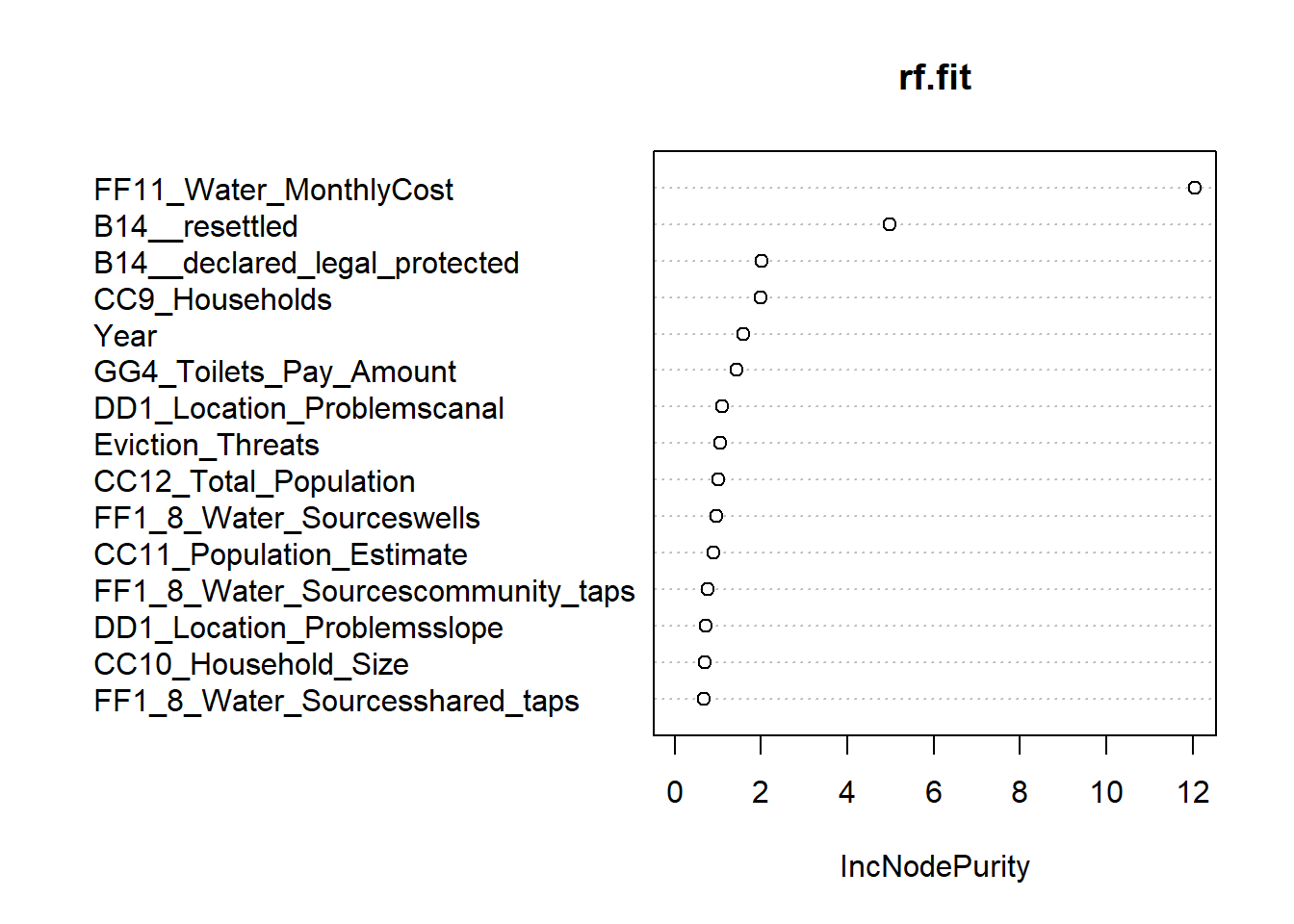
4. Lasso
Use library
glmnet.
Lasso is a shrinkage approach for feature selection. The tuning parameter lambda is the magnitudes of penalty. A increasing penalty shrinks coefficients towards zero. The advantage of a linear model is that the result is highly interpretable.We use cross-validation to choose the lambda and corresponding features
The dotted line on the left is lambda.min, the lambda that generates the lowest MSE in the testing dataset. The dotted line on the right is lambda.1se, its corresponding MSE is not the lowest but acceptable, and it has even fewer features in the model. We use
lambda.1sein our case.
# Use cross-validation to select the lambda
cv_lasso = cv.glmnet(X_train, Y_train, alpha=1) # Lasso regression
plot(cv_lasso)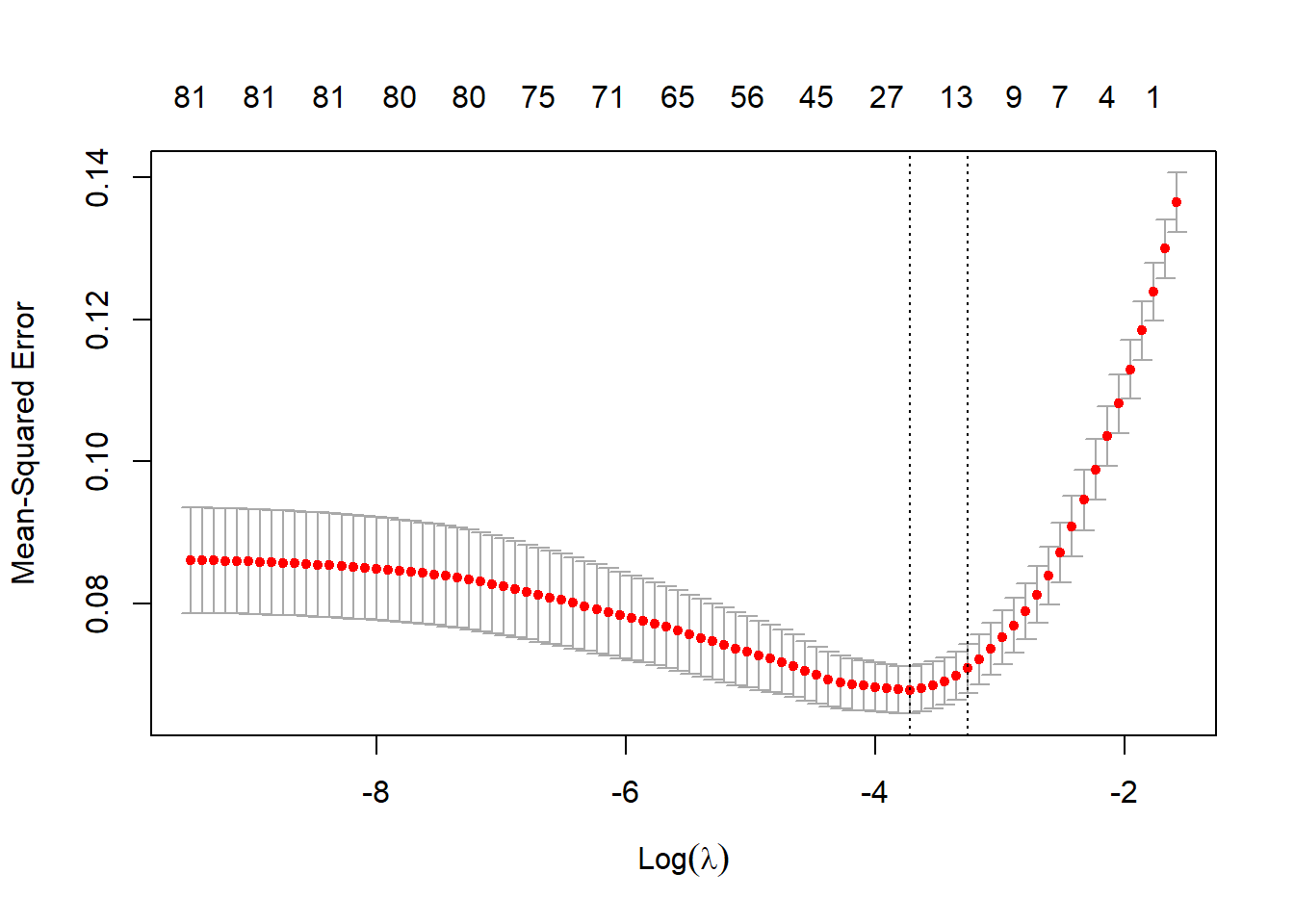
# lambda selected by 1se rule
(best_lam <- cv_lasso$lambda.1se)
## [1] 0.03845- MSE
# Check prediction error in the testing dataset
lasso_pred <- predict(lasso_mod, s = best_lam, newx = X_test)
# The Mean squared error (MSE)
(MSE_Lasso <- mean((lasso_pred - Y_test)^2))
## [1] 0.06751The regression model for the selected lambda (lasso). We extract the coefficients from the selected model and run a linear regression.
The model has used 17 variables.
The most useful predictors selected by lasso include
Water_MonthlyCost,Water_Sources: shared_taps,Resettled HousingandEviction Threats. For these variables, higher values or binary variables being Yes are associated with fewer temporary structures in slums.Relative importance of coefficients by showing standardized regression coefficients in decreasing order of their absolute values.
coef_table2 <- data.frame(reg_lasso_summary$coefficients, stb = c(0, lm.beta(reg_lasso_mod)))
coef_table2[order(abs(coef_table2$stb), decreasing = T),]
## Estimate Std..Error t.value Pr...t..
## B14__resettled -1.500e-01 3.232e-02 -4.641 4.404e-06
## DD1_Location_Problemscanal 1.896e-01 3.278e-02 5.785 1.261e-08
## FF11_Water_MonthlyCost -3.354e-06 6.940e-07 -4.832 1.788e-06
## FF1_8_Water_Sourceswells -1.146e-01 2.294e-02 -4.995 8.084e-07
## Eviction_Threats 1.053e-01 2.428e-02 4.337 1.736e-05
## B14__declared_legal_protected 8.688e-02 2.967e-02 2.928 3.561e-03
## DD1_Location_Problemsslope 8.235e-02 2.366e-02 3.481 5.422e-04
## EE2B_Current_Eviction_Seriousnessmedium -2.149e-01 6.549e-02 -3.282 1.101e-03
## GG1_Sewer_Line 7.801e-02 2.500e-02 3.120 1.908e-03
## FF1_8_Water_Sourceswater_tankers -1.203e-01 3.949e-02 -3.046 2.434e-03
## GG7_Managerprivate -5.983e-02 2.417e-02 -2.475 1.363e-02
## DD1_Location_Problemsflood_prone_area 4.860e-02 2.254e-02 2.156 3.152e-02
## FF1_8_Water_Sourcescommunity_taps 4.666e-02 2.929e-02 1.593 1.118e-01
## (Intercept) 3.949e-01 3.957e-02 9.979 1.479e-21
## stb
## B14__resettled -0.19503
## DD1_Location_Problemscanal 0.18221
## FF11_Water_MonthlyCost -0.17854
## FF1_8_Water_Sourceswells -0.15557
## Eviction_Threats 0.14234
## B14__declared_legal_protected 0.11390
## DD1_Location_Problemsslope 0.10926
## EE2B_Current_Eviction_Seriousnessmedium -0.10030
## GG1_Sewer_Line 0.09478
## FF1_8_Water_Sourceswater_tankers -0.09144
## GG7_Managerprivate -0.07741
## DD1_Location_Problemsflood_prone_area 0.06608
## FF1_8_Water_Sourcescommunity_taps 0.05158
## (Intercept) 0.000005. Best Subset
Use library
leaps.
Best subset is a subset selection approach for feature selection. Not like stepwise or forward selection, best subset check all the possible feature combinations in theory. Since I select from 49 predictors but set the maximum size of subsets to be 25, there are C(49,25) + C(49,24) + …+ C(49,0) = 345 trillion models to check. As I discussed in my post, it won’t be possible to scan all of them. Both R and SAS use the branch and bound algorithm to speed up the calculation.If without cross-validation we can use the traditional way to choose model: Adjusted R-squared, Cp(AIC), or BIC.
The turning parameter is to decide how many predictors to use. The selected number of feature also happens to be 17.
Cross-validation selects more features than BIC but fewer than Adj Rsq or Cp(AIC).The regression model selected and Standardized parameter estimates showing relative feature importance in decreasing order.
##                                       b.Estimate b.Std..Error b.t.value
## B14__resettled                        -2.275e-01    4.111e-02   -5.5342
## DD1_Location_Problemscanal             2.076e-01    4.235e-02    4.9029
## FF11_Water_MonthlyCost                -3.553e-06    9.722e-07   -3.6545
## Eviction_Threats                       1.227e-01    4.541e-02    2.7018
## B14__declared_legal_protected          1.203e-01    4.067e-02    2.9583
## FF1_8_Water_Sourceswater_tankers      -1.820e-01    5.533e-02   -3.2893
## FF1_8_Water_Sourcesshared_taps        -1.117e-01    4.894e-02   -2.2831
## DD1_Location_Problemsflood_prone_area  6.877e-02    3.054e-02    2.2516
## GG7_10_Toilet_Typesindividual_toilets -6.214e-02    4.268e-02   -1.4561
## FF1_8_Water_Sourcessprings            -5.563e-02    4.252e-02   -1.3085
## JJ1_Electricity_Availableyes           5.644e-02    4.699e-02    1.2012
## DD1_Location_Problemsgarbage_dump     -3.611e-02    3.347e-02   -1.0791
## EE2A_Current_Eviction_Threat           2.456e-02    4.528e-02    0.5425
## FF1_8_Water_Sourcesrivers             -4.108e-02    5.889e-02   -0.6976
## FF1_8_Water_Sourcesdams               -2.846e-02    7.258e-02   -0.3921
## FF12_Water_CollectionTime30_minutes    1.275e-02    4.478e-02    0.2847
## DD1_Location_Problemsroad_side        -1.899e-03    3.160e-02   -0.0601
## (Intercept)                            3.932e-01    7.437e-02    5.2871
##                                       b.Pr...t..       stb
## B14__resettled                         6.856e-08 -0.294884
## DD1_Location_Problemscanal             1.554e-06  0.205337
## FF11_Water_MonthlyCost                 3.044e-04 -0.185969
## Eviction_Threats                       7.293e-03  0.164439
## B14__declared_legal_protected          3.341e-03  0.156849
## FF1_8_Water_Sourceswater_tankers       1.125e-03 -0.135517
## FF1_8_Water_Sourcesshared_taps         2.313e-02 -0.096201
## DD1_Location_Problemsflood_prone_area  2.508e-02  0.093098
## GG7_10_Toilet_Typesindividual_toilets  1.464e-01 -0.058293
## FF1_8_Water_Sourcessprings             1.917e-01 -0.056320
## JJ1_Electricity_Availableyes           2.306e-01  0.050303
## DD1_Location_Problemsgarbage_dump      2.814e-01 -0.044732
## EE2A_Current_Eviction_Threat           5.879e-01  0.031196
## FF1_8_Water_Sourcesrivers              4.860e-01 -0.027726
## FF1_8_Water_Sourcesdams                6.953e-01 -0.015868
## FF12_Water_CollectionTime30_minutes    7.760e-01  0.011364
## DD1_Location_Problemsroad_side         9.521e-01 -0.002456
## (Intercept) 2.408e-07 0.000000- MSE
## [1] 0.06979Compare MSEs
The advantage of XGboost is highly distinguishing.
- XGBoost shows advantage in rmse but not too distinguishing
- XGBoost’s real advantages include its speed and ability to handle missing values
##   MSE_xgb MSE_boost MSE_Lasso MSE_rForest MSE_best.subset
## 1 0.04237   0.04838   0.06751     0.04359         0.06979