1.1. US Map (50 states) using usmap

The easiest way is by using usmap, in which adding abbraviation or not is optional in the plot_usmap function. The population data is from state.x77, data of a US census in 1977.

#51 states including Alaska and Hawaii
suppressPackageStartupMessages({
library(ggplot2)
library(maps)
library(usmap)
library(data.table)
library(ggsn) # for scale bar `scalebar`
library(ggrepel) # if need to repel labels 
})
dt1 <- as.data.table(copy(state.x77))
dt1$state <- tolower(rownames(state.x77))
dt1 <- dt1[,.(state, Population)]
# only need state name and variable to plot in the input file:
str(dt1) 

## Classes 'data.table' and 'data.frame':   50 obs. of  2 variables:
##  $ state     : chr  "alabama" "alaska" "arizona" "arkansas" ...
##  $ Population: num  3615 365 2212 2110 21198 ...
##  - attr(*, ".internal.selfref")=<externalptr>

us_map <- usmap::us_map() # used to add map scale

usmap::plot_usmap(data = dt1, values = "Population", labels = T)+
  labs(fill = 'State Population (1975)') + 
  scale_fill_gradientn(colours=rev(heat.colors(10)),na.value="grey90",
                       guide = guide_colourbar(barwidth = 25, barheight = 0.4,
                                               #put legend title on top of legend
                                               title.position = "top")) +
  # map scale
  ggsn::scalebar(data = us_map, dist = 500, dist_unit = "km",
           border.size = 0.4, st.size = 4,
           box.fill = c('black','white'),
           transform = FALSE, model = "WGS84") + 
  # put legend at the bottom, adjust legend title and text font sizes
  theme(legend.position = "bottom",
        legend.title=element_text(size=12), 
        legend.text=element_text(size=10))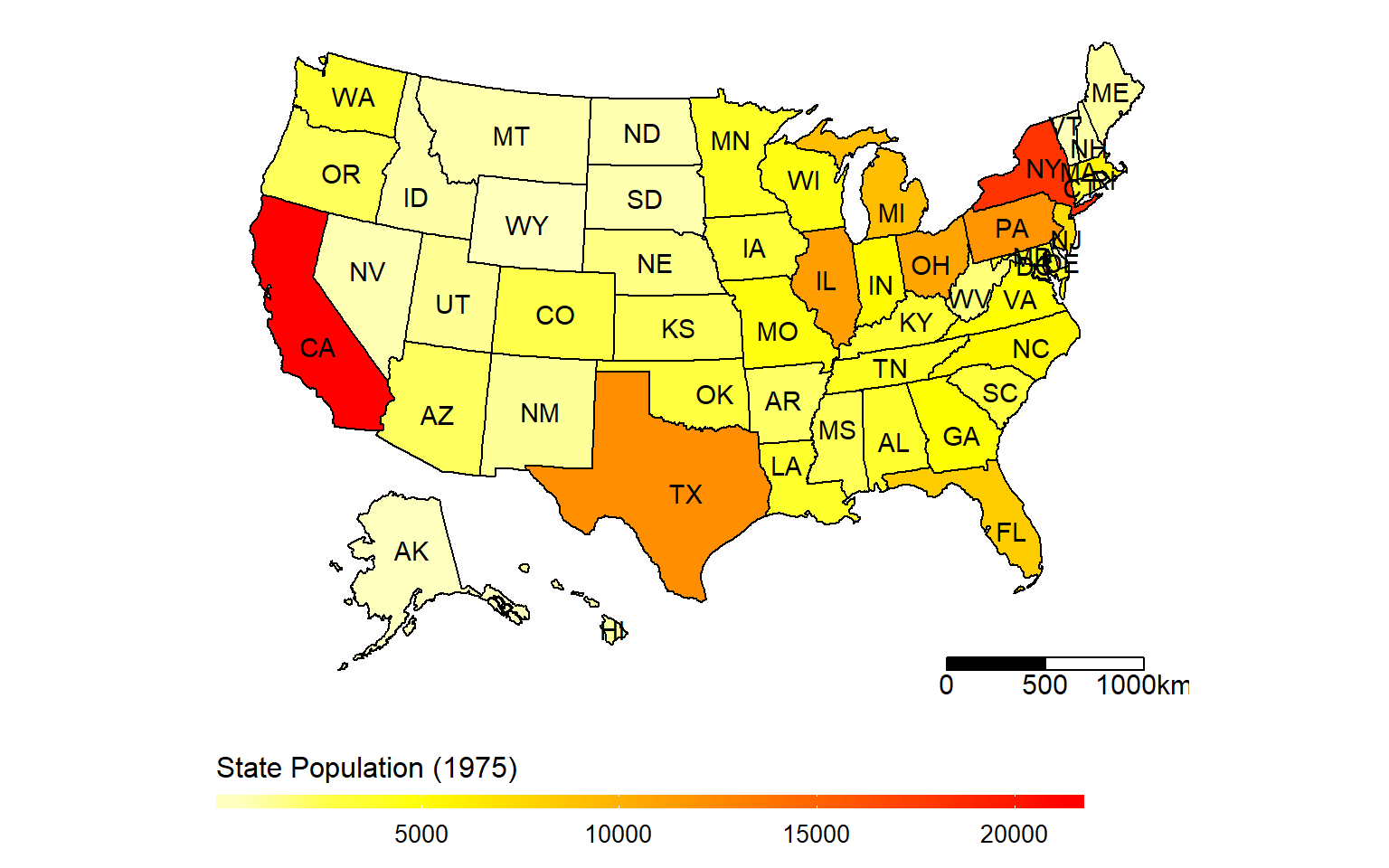

The plot_usmap returns a ggplot object so it is possible to further revise by just adding more layers.

1.2. Using map_data and build from scratch

Could fine-tune the location of states’label as I did in the China map later. Now it is just the center of the states (mean(lon), min(lat))

dt2 <- as.data.table(copy(state.x77))
dt2$state <- tolower(rownames(state.x77))
dt2 <- dt2[,.(state, Population)]
setkey(dt2, state)

states <- setDT(ggplot2::map_data("state"))
setkey(states, region)
# join data to map: left join states to dt2
dt2 <- dt2[states]
# data look like this: 
rmarkdown::paged_table(dt2[1:500,])

# create states location and abbreviations for label
# incl `Population` (the value to plot) in the label dataset, if want to fill with color. 
state_label_dt <- unique(dt2[, .(Population, x = mean(range(long)), y = mean(range(lat))), by = state])
snames <- data.table(state = tolower(state.name), abb = state.abb) # these are dataset within R
setkey(state_label_dt, state)
setkey(snames, state)
state_label_dt <- snames[state_label_dt]


# All labels for states to the right of lon = -77 will be on the right of lon = -50.
x_boundary = -77
x_limits <- c(-50, NA) # optional, for label repelling

ggplot(data = dt2, aes(x=long, y=lat, group=group))+
  geom_polygon(aes(fill=Population))+
  geom_path()+ 
  scale_fill_gradientn(colours = rev(heat.colors(10)),na.value = "grey90",
                       guide = guide_colourbar(barwidth = 25, barheight = 0.4,
                                               #put legend title on top of legend
                                               title.position = "top")) +
  # if need to repel labels... could further finetune
  geom_label_repel(data = state_label_dt[x>=x_boundary,],
                   aes(x = x,y = y, label = abb, fill = Population),
    arrow = arrow(length = unit(0.02, "npc"), ends = "first"),
    force = 5, hjust = 1, size = 3,
    xlim  = x_limits, inherit.aes = F
  ) +
  # the normal labels: 
  geom_text(data=state_label_dt[x<x_boundary,], aes(x=x,y=y, label=abb), 
            size=3, inherit.aes=F) +
  coord_map() + 
  theme_classic() + 
  labs(fill = "Population", x = "Longitude", y = "Latitude") + 

    # map scale
  ggsn::scalebar(data = dt2, dist = 500, dist_unit = "km",
           border.size = 0.4, st.size = 4,
           box.fill = c('black','white'),
           transform = TRUE, model = "WGS84") + 
  # put legend at the bottom, adjust legend title and text font sizes
  theme(legend.position = "bottom",
        legend.title=element_text(size=12),  # font size of the legend 
        legend.text=element_text(size=10),
        axis.title.x=element_blank(),  # remove axis, title, ticks
        axis.text.x=element_blank(),
        axis.ticks.x=element_blank(),
        axis.line=element_blank())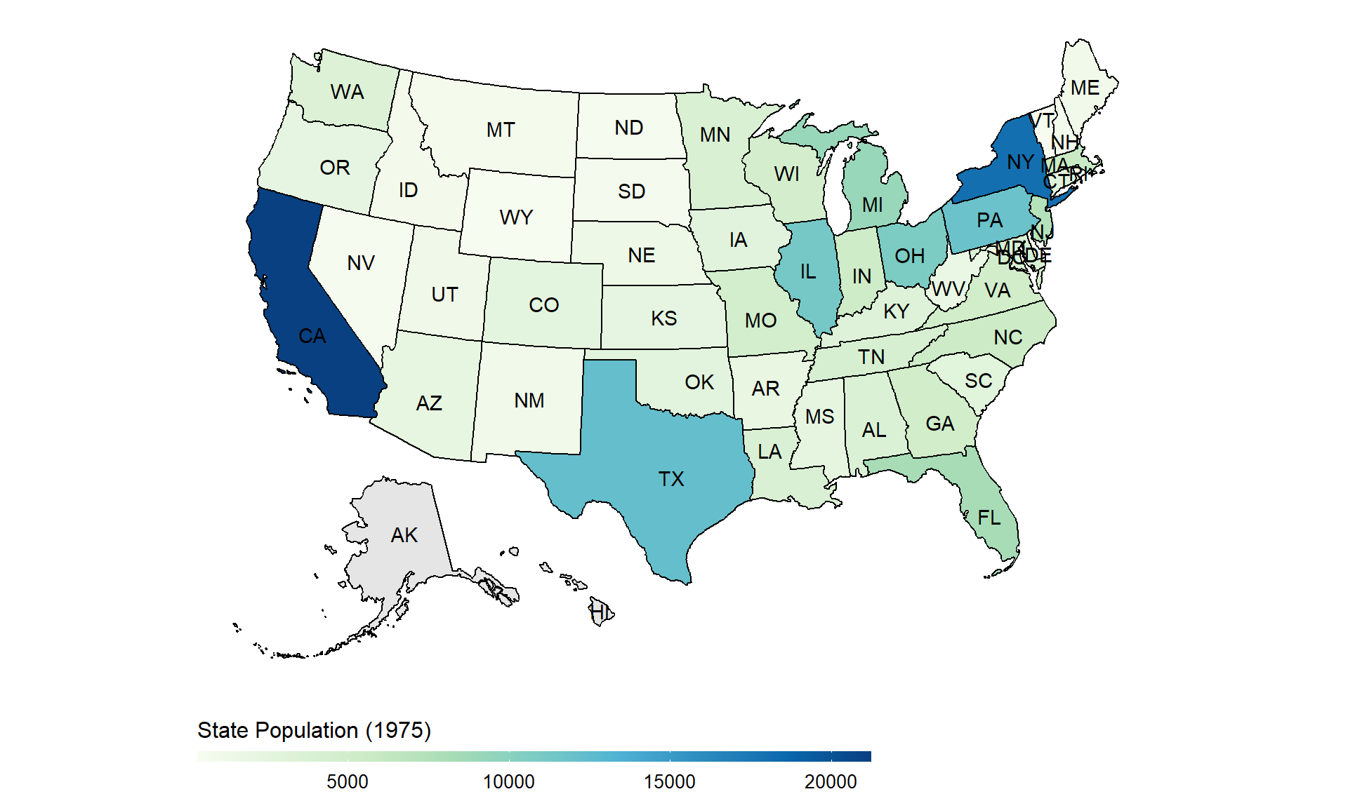

2.1. China map by province using downloaded shapfiles

The map of China is more complicated. The related articles are all from several years ago. This blog by Zhang, Zhen is among the best, it has referred some very good resources, expecially this one on Capital Of Statistics (CH)](https://cosx.org/2009/07/drawing-china-map-using-r). This is a blog from 10 years ago. So far there is still no map package for China like usmap.

The shape files need to be downloaded from the “Capital of Statistics” webiste, the zip file contains three files: bou2_4p.dbf, bou2_4p.shp, and bou2_4p.shx, we will load the shp file later.

Printing Chinese is indeed sometimes a problem. The key is to aline in the datafile all the chinese are in UTF-8. In the markdown file below you can see Chinese characters are actually shown as UTF-8 code. But in the map (plot) they are rendered correctly.

一点额外说明

我用的是Windows系统，只要Rstudio中显示中文没有问题好像Markdown中文就没有太大问题。关键是要统一数据中的中文都是UTF-8编码的，不要从网站上拷贝中文进Rstudio，会产生各种问题。不需要特别调整Rstudio或者Markdown的设置。

所以虽然我下面的数据中显示UTF-8，最后在地图上是可以显示中文的。 参考的统计之都上的博客都是十年前的了。希望将来能看到mapchina package的出现。

# China -------------------------------------------------------------------
library(maptools)
local_fir_dir <- "D:/OneDrive/David/China.shp/" # local the .shp file is stored  
china_map <- rgdal::readOGR(paste0(local_fir_dir, "bou2_4p.shp"))

## OGR data source with driver: ESRI Shapefile 
## Source: "D:\OneDrive\David\China.shp\bou2_4p.shp", layer: "bou2_4p"
## with 925 features
## It has 7 fields
## Integer64 fields read as strings:  BOU2_4M_ BOU2_4M_ID

# extract province information from shap file
china_province = setDT(china_map@data)
setnames(china_province, "NAME", "province")

# transform to UTF-8 coding format
china_province[, province:=iconv(province, from = "GBK", to = "UTF-8")] 
# create id to join province back to lat and long, id = 0 ~ 924
china_province[, id:= .I-1] 
# there are more shapes for one province due to small islands
china_province[, table(province)]

## province
## <U+4E0A><U+6D77><U+5E02> <U+4E91><U+5357><U+7701> <U+5185><U+8499><U+53E4><U+81EA><U+6CBB><U+533A> <U+5317><U+4EAC><U+5E02> 
##               12                1                1                1 
## <U+53F0><U+6E7E><U+7701> <U+5409><U+6797><U+7701> <U+56DB><U+5DDD><U+7701> <U+5929><U+6D25><U+5E02> 
##               57                1                1                1 
## <U+5B81><U+590F><U+56DE><U+65CF><U+81EA><U+6CBB><U+533A> <U+5B89><U+5FBD><U+7701> <U+5C71><U+4E1C><U+7701> <U+5C71><U+897F><U+7701> 
##                1                1               86                1 
## <U+5E7F><U+4E1C><U+7701> <U+5E7F><U+897F><U+58EE><U+65CF><U+81EA><U+6CBB><U+533A> <U+65B0><U+7586><U+7EF4><U+543E><U+5C14><U+81EA><U+6CBB><U+533A> <U+6C5F><U+82CF><U+7701> 
##              154                6                1                5 
## <U+6C5F><U+897F><U+7701> <U+6CB3><U+5317><U+7701> <U+6CB3><U+5357><U+7701> <U+6D59><U+6C5F><U+7701> 
##                1                9                1              179 
## <U+6D77><U+5357><U+7701> <U+6E56><U+5317><U+7701> <U+6E56><U+5357><U+7701> <U+7518><U+8083><U+7701> 
##               79                1                1                1 
## <U+798F><U+5EFA><U+7701> <U+897F><U+85CF><U+81EA><U+6CBB><U+533A> <U+8D35><U+5DDE><U+7701> <U+8FBD><U+5B81><U+7701> 
##              168                1                2               94 
## <U+91CD><U+5E86><U+5E02> <U+9655><U+897F><U+7701> <U+9752><U+6D77><U+7701> <U+9999><U+6E2F><U+7279><U+522B><U+884C><U+653F><U+533A> 
##                1                1                1               53 
## <U+9ED1><U+9F99><U+6C5F><U+7701> 
##                1

china_province[, province:= as.factor(province)]

dt_china = setDT(fortify(china_map))
dt_china[, id:= as.numeric(id)]

setkey(china_province, id); setkey(dt_china, id)
dt_china <- china_province[dt_china]

# make the province EN, CH label file
province_CH <- china_province[, levels(province)] # the CH are in UTF-8 code
province_EN <- c("Shanghai", "Yunnan", "Inner Mongolia", "Beijing", "Taiwan",
"Jilin", "Sichuan", "Tianjin City", "Ningxia", "Anhui",
"Shandong", "Shanxi", "Guangdong", "Guangxi ", "Xinjiang",
"Jiangsu", "Jiangxi", "Hebei", "Henan", "Zhejiang",
"Hainan", "Hubei", "Hunan", "Gansu", "Fujian",
"Tibet", "Guizhou", "Liaoning", "Chongqing", "Shaanxi",
"Qinghai", "Hong Kong", "Heilongjiang"
)

# some population data (from years ago too)
value <- c(8893483, 12695396,  8470472,  7355291, 23193638,  9162183, 26383458,  3963604,  1945064, 19322432, 30794664, 10654162, 32222752, 13467663,  6902850, 25635291, 11847841, 20813492, 26404973, 20060115, 2451819, 17253385, 19029894,  7113833, 11971873,   689521, 10745630, 15334912, 10272559, 11084516, 1586635,  7026400, 13192935)
input_data <- data.table(province_CH, province_EN, value)
setkey(input_data, province_CH)
setkey(dt_china, province)

# remove small islands on the South China Sea
china_map_pop <- input_data[dt_china[AREA>0.1,]]

# create label file of province `label_dt`
label_dt <- china_map_pop[, .(x = mean(range(long)), y = mean(range(lat)), province_EN, province_CH), by = id]
label_dt <- unique(label_dt)
setkey(label_dt, province_EN)
# I have fine-tuned the label position of some provinces
label_dt['Inner Mongolia', `:=` (x = 110, y = 42)]
label_dt['Gansu', `:=` (x = 96.3, y = 40)]
label_dt['Hebei', `:=` (x = 115.5, y = 38.5)]
label_dt['Liaoning', `:=` (x = 123, y = 41.5)]

# data look like this: 
rmarkdown::paged_table(china_map_pop[!is.na(province_CH),])

# plot
ggplot(china_map_pop, aes(x = long, y = lat, group = group, fill=value)) +
  labs(fill = "Population (outdated)")+
  geom_polygon()+
  geom_path()+
  scale_fill_gradientn(colours=rev(heat.colors(10)),na.value="grey90",
                       guide = guide_colourbar(barwidth = 0.8, barheight = 10)) + 
  blank() + 
  geom_text(data = label_dt, aes(x=x, y=y, label = province_EN),inherit.aes = F) +
  scalebar(data = china_map_pop, dist = 500, dist_unit = "km",
           transform = T, model = "WGS84",
           border.size = 0.4, st.size = 2)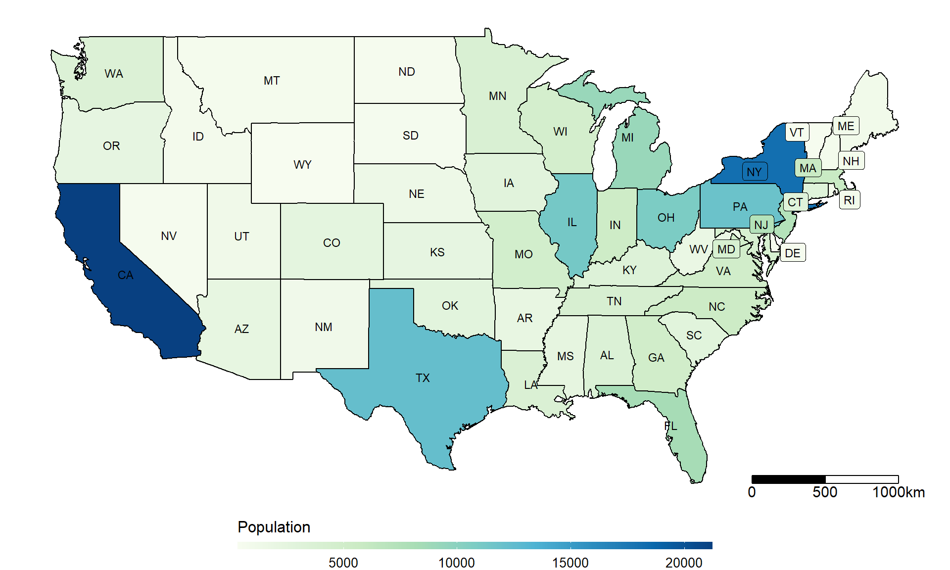 

ggplot(china_map_pop, aes(x = long, y = lat, group = group, fill=value)) +
  labs(fill = "Population")+
  geom_polygon()+
  geom_path()+
  scale_fill_gradientn(colours=rev(heat.colors(10)),na.value="grey90") + 
  blank() + 
  geom_text(data = label_dt, aes(x=x, y=y, label = province_CH),inherit.aes = F) +
  scalebar(data = china_map_pop, dist = 500, dist_unit = "km",
           transform = T, model = "WGS84",
           border.size = 0.4, st.size = 2)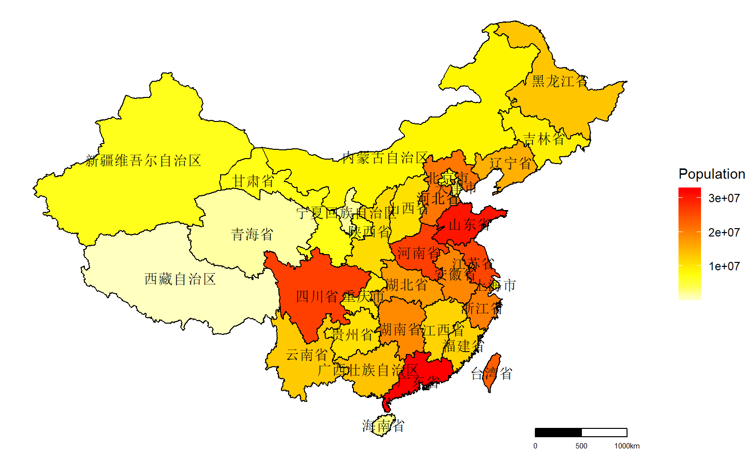 

2.2. Using geojsonMap (leaflet)

Just saw it on cosx.org blog. It is an interactive map built on leaflet.

library(leafletCN)
china_map_pop <- as.data.frame(china_map_pop)
geojsonMap(dat = china_map_pop, mapName = "china",
           namevar = ~ province_CH, valuevar = ~ value, 
           popup =  paste0(china_map_pop$province_EN),
           palette = "Reds", legendTitle = "Population")

Moreover, it is possible to get China’s map_data from maps (ggplot2), as we did with the US map. But I don’t think it has province information associated.(to be further investigated)

dt3 <- ggplot2::map_data("china")
ggplot(dt3, aes(long, lat, group=group, fill=region)) +
  geom_path(show.legend = F)
head(dt3)