Drake: powerful tool for automatic reproducible workflow

drake is a powerful tool for automatic reproducible workflow. I found it a perfect match when used together with RMarkdown. There are great documentations online for drake thus here I only show a simple example working with RMarkdown.

RMarkdown file could be very slow to generate if lots of calculations are involved. Any small revise makes you rerun everything. When we use drake we can do all the calculations in advance thus the rendering is super fast since we only need to re-do the revised object.

Using SHAPforxgboost as an example:

# if needed, update drake
if(packageVersion("drake") < "7.4") install.packages("drake")
if(packageVersion("SHAPforxgboost") < "0.0.3") install.packages("SHAPforxgboost")

suppressPackageStartupMessages({
  library("drake")
  library("SHAPforxgboost")
  library("here")
})

# assign a place to store intermediate objects
cache_path <- here("Drake_Cache")
if(!dir.exists(cache_path))dir.create(cache_path)
cache <- drake_cache(path = cache_path)

The drake_plan takes self-defined functions to create each target. All the functions are usually written in a seperate script.

get.xgb.mod <- function(dataX){
  y_var <- "diffcwv" 
  # hyperparameter tuning results
  param_dart <- list(objective = "reg:linear",  # For regression
                   nrounds = 366,
                   eta = 0.018,
                   max_depth = 10,
                   gamma = 0.009,
                   subsample = 0.98,
                   colsample_bytree = 0.86)

  mod <- xgboost::xgboost(data = as.matrix(dataX), 
                        label = as.matrix(dataXY_df[[y_var]]), 
                       xgb_param = param_dart, nrounds = param_dart$nrounds,
                       verbose = FALSE, nthread = parallel::detectCores() - 2,
                       early_stopping_rounds = 8)
  return(mod)
}

# ...
# define more functions if needed
# ...

Markdown all the results to the final report. The great advantage is that since all the figures were done and stored before the markdown process, if you modify a figure, only that figure needs to be rerun.

my_plan <- drake_plan(
  dataX = data.table::copy(dataXY_df[,-"diffcwv"]),
  xgb_mod = get.xgb.mod(dataX),
  shap_long = shap.prep(xgb_model = xgb_mod, X_train = dataX, top_n = 4),
  # make a diluted (faster) summary plot showing only top 4 variables:
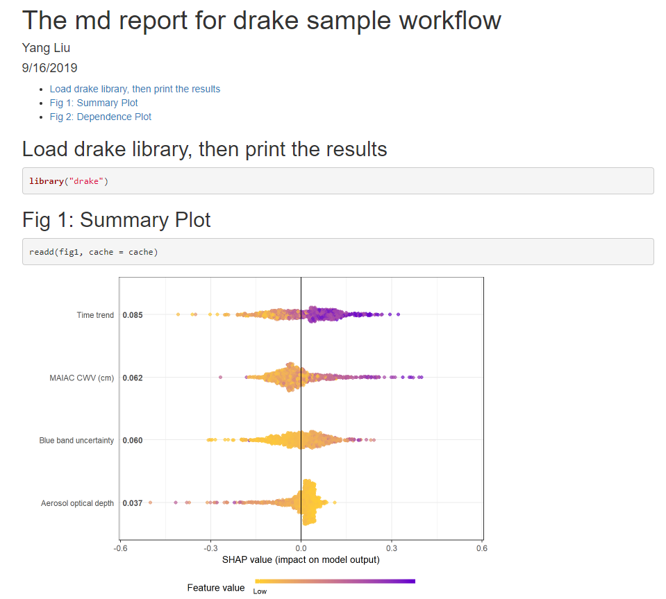
  fig1 = shap.plot.summary(shap_long, dilute = 10),
  fig2 = shap.plot.dependence(data_long = shap_long, x = 'dayint', y = 'dayint', color_feature = 'Column_WV'),
  fig3 = shap.plot.dependence(data_long = shap_long, x = 'dayint', y = 'Column_WV', color_feature = 'Column_WV'),
  
  report = `RMarkdown`::render(
    knitr_in("Code/drake_md_report.Rmd"),
    output_format = `RMarkdown`::html_document(toc = TRUE))
)

nemia_config <- drake_config(my_plan, cache = cache) # show the dependency
# vis_drake_graph(nemia_config, from = names(nemia_config$layout))
vis_drake_graph(nemia_config)

# run the plan
make(my_plan, cache = cache)

Notice that it is not a good idea to run drake within a RMarkdown file as drake workflow should be an R script that uses RMarkdown as the output tool. So I cannot really render this post as it is. But these code can run as

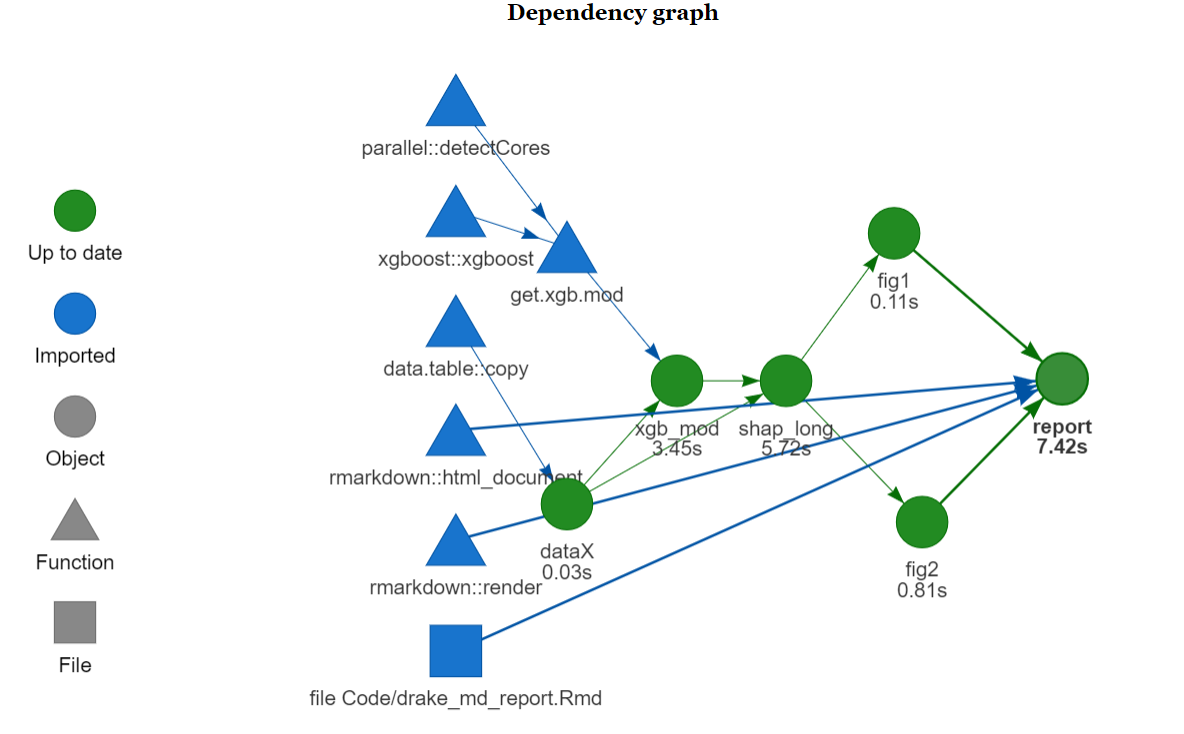
Here is how the dependency graph looks like:

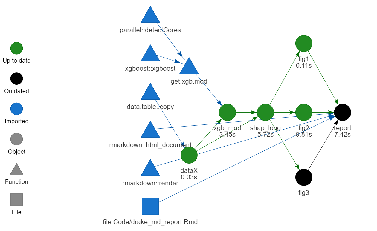
If we add an extra figure, only this figure (the black fig3) needs to made:

Here is how the md file looks like on Github

And the drake work plan generates a markdown results automatcially (“drake_md_report.html”) which looks like this:

Drake: powerful tool for automatic reproducible workflow

Yang Liu