---
title: "eXtreme Gradient Boosting (XGBoost): Better than random forest or gradient boosting"
author: "Yang Liu"
date: "2018-07-09"
description: "A hands-on R comparison of XGBoost, gradient boosting, random forest, lasso, and best subset regression on a slum-settlement modeling example."
categories:
- "Machine Learning"
tags:
- "XGBoost"
page-layout: article
execute:
freeze: true
eval: false
resources:
- "source.Rmd"
- "index_files/**"
- "images/**"
- "temp/**"
- "2018-07-09-extreme-gradient-boosting-xgboost-better-than-random-forest-or-gradient-boosting_files/**"
- "*.png"
- "*.jpg"
- "*.jpeg"
- "*.JPG"
- "*.PNG"
- "*.gif"
- "*.svg"
- "*.rds"
- "*.csv"
- "*.xlsx"
---
<script src="../../rmarkdown-libs/header-attrs/header-attrs.js"></script>
<script src="../../rmarkdown-libs/htmlwidgets/htmlwidgets.js"></script>
<script src="../../rmarkdown-libs/viz/viz.js"></script>
<link href="../../rmarkdown-libs/DiagrammeR-styles/styles.css" rel="stylesheet" />
<script src="../../rmarkdown-libs/grViz-binding/grViz.js"></script>
<div id="TOC">
<ul>
<li><a href="#overview">Overview</a></li>
<li><a href="#about-the-data">About the Data</a></li>
<li><a href="#extreme-gradient-boosting">1. Extreme Gradient Boosting</a></li>
<li><a href="#gradient-boosting">2. Gradient boosting</a></li>
<li><a href="#random-forest">3. Random Forest</a></li>
<li><a href="#lasso">4. Lasso</a></li>
<li><a href="#best-subset">5. Best Subset</a></li>
<li><a href="#compare-mse">Compare MSE</a></li>
</ul>
</div>
<div id="overview" class="section level1">
<h1>Overview</h1>
<p>I first learned about eXtreme Gradient Boosting (XGBoost) from Professor Allan Just, then extended an earlier modeling exercise <a href="https://yangliuresearch.blogspot.com/2018/06/modeling-of-slums-model-selection-using.html">from my old blog</a> by comparing XGBoost, Gradient Boosting (GBM), Random Forest, Lasso, and Best Subset regression.</p>
<p>Ensemble methods are powerful because they combine many weaker predictions into a stronger model. Random Forest averages many decorrelated decision trees built from bootstrap samples. Boosting works sequentially: each new tree focuses on the residual patterns left by the previous trees.</p>
<p><strong>Correction, 2018-10-03:</strong> my first version reported a testing error almost ten times smaller than the other methods. That was a mistake. In the corrected result, XGBoost still had the lowest testing RMSE, but it was close to the other tree-based methods.</p>
<p>Link to the earlier version: <a href="https://yangliuresearch.blogspot.com/2018/06/modeling-of-slums-model-selection-using.html"><em>Model Selection using Lasso and Best Subset</em></a></p>
</div>
<div id="about-the-data" class="section level1">
<h1>About the Data</h1>
<p>In sub-Saharan Africa, where deprivations in living conditions are especially severe, slum dwellers represent an estimated 56% of the region's urban population (UN Habitat, 2016). Measuring informal settlements reliably is a critical challenge for monitoring the Sustainable Development Goals (SDGs). The data in this example were collected by Slum Dwellers International (SDI), which was nominated for the Nobel Peace Prize in 2014.</p>
<p>In this exercise, we only model <em>Share_Temporary</em>: Share of Temporary Structure in Slums as the dependent variable. The independent variables are monitoring indicators like water, sanitation, housing conditions and overcrowding in African slum settlements. Dataset dimension is 973 x 153.</p>
</div>
<div id="extreme-gradient-boosting" class="section level1">
<h1>1. Extreme Gradient Boosting</h1>
<ul>
<li>Random search: randomized parameters and update the record with best ones.</li>
<li>It turns out to be a very interesting method to scan for hyperparameters. It will take a while for 100 iterations.</li>
<li>The package <code>xgboost</code> is really fast.</li>
</ul>
<pre class="r"><code>library(xgboost)
# Randomize and bound
best_param <- list()
best_seednumber <- 1234
best_rmse <- Inf
best_rmse_index <- 0
set.seed(1234)
# In reality, might need 100 or 200 iterations
for (iter in 1:10) {
param <- list(objective = "reg:squarederror", # For regression
eval_metric = "rmse", # rmse is used for regression
max_depth = sample(6:10, 1),
eta = runif(1, .01, .1), # Learning rate, default: 0.3
subsample = runif(1, .6, .9),
colsample_bytree = runif(1, .5, .8),
min_child_weight = sample(5:10, 1), # These two are important
max_delta_step = sample(5:10, 1) # Can help to focus error
# into a small range.
)
cv.nround <- 1000
cv.nfold <- 5 # 5-fold cross-validation
seed.number <- sample.int(10000, 1) # set seed for the cv
set.seed(seed.number)
mdcv <- xgb.cv(data = dtrain, params = param,
nfold = cv.nfold, nrounds = cv.nround,
verbose = F, early_stopping_rounds = 8, maximize = FALSE)
min_rmse_index <- mdcv$best_iteration
min_rmse <- mdcv$evaluation_log[min_rmse_index]$test_rmse_mean
if (min_rmse < best_rmse) {
best_rmse <- min_rmse
best_rmse_index <- min_rmse_index
best_seednumber <- seed.number
best_param <- param
}
}</code></pre>
<ul>
<li>The best tuning parameters<br />
</li>
</ul>
<pre><code>## objective eval_metric max_depth eta subsample colsample_bytree
## 1 reg:squarederror rmse 9 0.09822 0.64 0.6853
## min_child_weight max_delta_step best_rmse_index best_rmse best_seednumber
## 1 6 8 56 0.2102 3660</code></pre>
<ul>
<li>MSE<br />
</li>
</ul>
<pre><code>## [1] 0.04237</code></pre>
<ul>
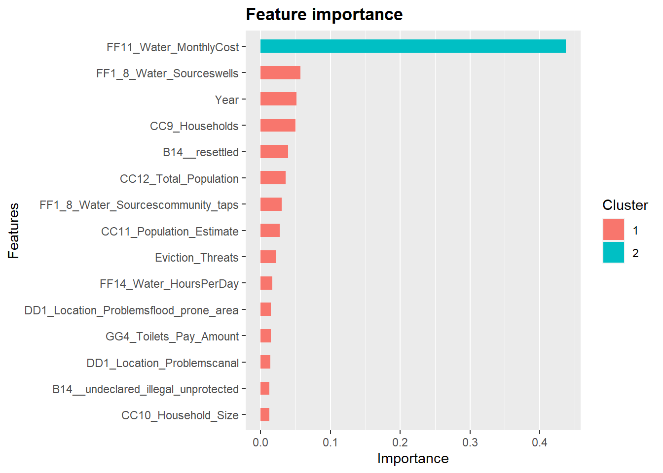
<li>Feature Importance<br />
</li>
</ul>
<pre class="r"><code>importance_matrix <- xgb.importance(feature_names = colnames(X_train),
model = xg_mod)
# Use `xgb.plot.importance`, which create a _barplot_ or use `xgb.ggplot.importance`
library(Ckmeans.1d.dp) # for xgb.ggplot.importance
xgb.ggplot.importance(importance_matrix, top_n = 15, measure = "Gain")</code></pre>
<p><img src="2018-07-09-extreme-gradient-boosting-xgboost-better-than-random-forest-or-gradient-boosting_files/figure-html/unnamed-chunk-4-1.png" width="672" /></p>
<ul>
<li>Plot only 2 trees as an example (use <code>trees</code>= 1)<br />
</li>
</ul>
<pre class="r"><code>library("DiagrammeR")
xgb.plot.tree(model = xg_mod, trees = 1, feature_names = colnames(X_train))</code></pre>
<div id="htmlwidget-033cbf18e5e6884abee8" style="width:672px;height:480px;" class="grViz html-widget"></div>
<script type="application/json" data-for="htmlwidget-033cbf18e5e6884abee8">{"x":{"diagram":"digraph {\n\ngraph [layout = \"dot\",\n rankdir = \"LR\"]\n\nnode [color = \"DimGray\",\n style = \"filled\",\n fontname = \"Helvetica\"]\n\nedge [color = \"DimGray\",\n arrowsize = \"1.5\",\n arrowhead = \"vee\",\n fontname = \"Helvetica\"]\n\n \"1\" [label = \"Tree 1\nFF11_Water_MonthlyCost\nCover: 201\nGain: 8.01718044\", shape = \"rectangle\", fontcolor = \"black\", fillcolor = \"Beige\"] \n \"2\" [label = \"FF11_Water_MonthlyCost\nCover: 68\nGain: 2.5171988\", shape = \"rectangle\", fontcolor = \"black\", fillcolor = \"Beige\"] \n \"3\" [label = \"FF1_8_Water_Sourcescommunity_taps\nCover: 133\nGain: 1.12723732\", shape = \"rectangle\", fontcolor = \"black\", fillcolor = \"Beige\"] \n \"4\" [label = \"FF12_Water_CollectionTime5_minutes\nCover: 17\nGain: 0.543181658\", shape = \"rectangle\", fontcolor = \"black\", fillcolor = \"Beige\"] \n \"5\" [label = \"FF1_8_Water_Sourceswells\nCover: 51\nGain: 0.559164047\", shape = \"rectangle\", fontcolor = \"black\", fillcolor = \"Beige\"] \n \"6\" [label = \"FF1_8_Water_Sourceswells\nCover: 100\nGain: 0.4103508\", shape = \"rectangle\", fontcolor = \"black\", fillcolor = \"Beige\"] \n \"7\" [label = \"EE2B_Current_Eviction_Seriousnesshigh\nCover: 33\nGain: 0.382634193\", shape = \"rectangle\", fontcolor = \"black\", fillcolor = \"Beige\"] \n \"8\" [label = \"Leaf\nCover: 7\nValue: 0.00300397468\", shape = \"oval\", fontcolor = \"black\", fillcolor = \"Khaki\"] \n \"9\" [label = \"Leaf\nCover: 10\nValue: -0.0316009298\", shape = \"oval\", fontcolor = \"black\", fillcolor = \"Khaki\"] \n \"10\" [label = \"GG4_Toilets_Pay_Amount\nCover: 36\nGain: 0.0622627735\", shape = \"rectangle\", fontcolor = \"black\", fillcolor = \"Beige\"] \n \"11\" [label = \"DD2_Location_Dangerous\nCover: 15\nGain: 0.204182982\", shape = \"rectangle\", fontcolor = \"black\", fillcolor = \"Beige\"] \n \"12\" [label = \"CC12_Total_Population\nCover: 42\nGain: 0.128097773\", shape = \"rectangle\", fontcolor = \"black\", fillcolor = \"Beige\"] \n \"13\" [label = \"B14__resettled\nCover: 58\nGain: 0.17589283\", shape = \"rectangle\", fontcolor = \"black\", fillcolor = \"Beige\"] \n \"14\" [label = \"CC11_Population_Estimate\nCover: 25\nGain: 0.155959845\", shape = \"rectangle\", fontcolor = \"black\", fillcolor = \"Beige\"] \n \"15\" [label = \"Leaf\nCover: 8\nValue: 0.00698826462\", shape = \"oval\", fontcolor = \"black\", fillcolor = \"Khaki\"] \n \"16\" [label = \"CC12_Total_Population\nCover: 22\nGain: 0.0130501986\", shape = \"rectangle\", fontcolor = \"black\", fillcolor = \"Beige\"] \n \"17\" [label = \"Leaf\nCover: 14\nValue: 0.0384371951\", shape = \"oval\", fontcolor = \"black\", fillcolor = \"Khaki\"] \n \"18\" [label = \"Leaf\nCover: 9\nValue: -0.00146562792\", shape = \"oval\", fontcolor = \"black\", fillcolor = \"Khaki\"] \n \"19\" [label = \"Leaf\nCover: 6\nValue: 0.0207516421\", shape = \"oval\", fontcolor = \"black\", fillcolor = \"Khaki\"] \n \"20\" [label = \"Leaf\nCover: 24\nValue: -0.0289320275\", shape = \"oval\", fontcolor = \"black\", fillcolor = \"Khaki\"] \n \"21\" [label = \"CC11_Population_Estimate\nCover: 18\nGain: 0.242588937\", shape = \"rectangle\", fontcolor = \"black\", fillcolor = \"Beige\"] \n \"22\" [label = \"FF12_Water_CollectionTime5_minutes\nCover: 14\nGain: 0.324621856\", shape = \"rectangle\", fontcolor = \"black\", fillcolor = \"Beige\"] \n \"23\" [label = \"Leaf\nCover: 44\nValue: -0.0416171513\", shape = \"oval\", fontcolor = \"black\", fillcolor = \"Khaki\"] \n \"24\" [label = \"Leaf\nCover: 10\nValue: -0.0260489751\", shape = \"oval\", fontcolor = \"black\", fillcolor = \"Khaki\"] \n \"25\" [label = \"FF1_8_Water_Sourceswells\nCover: 15\nGain: 0.170917317\", shape = \"rectangle\", fontcolor = \"black\", fillcolor = \"Beige\"] \n \"26\" [label = \"CC11_Population_Estimate\nCover: 13\nGain: 0.171785772\", shape = \"rectangle\", fontcolor = \"black\", fillcolor = \"Beige\"] \n \"27\" [label = \"Leaf\nCover: 9\nValue: 0.0308628436\", shape = \"oval\", fontcolor = \"black\", fillcolor = \"Khaki\"] \n \"28\" [label = \"Leaf\nCover: 9\nValue: -0.00386937149\", shape = \"oval\", fontcolor = \"black\", fillcolor = \"Khaki\"] \n \"29\" [label = \"Leaf\nCover: 9\nValue: -0.0266056787\", shape = \"oval\", fontcolor = \"black\", fillcolor = \"Khaki\"] \n \"30\" [label = \"Leaf\nCover: 7\nValue: -0.00815664604\", shape = \"oval\", fontcolor = \"black\", fillcolor = \"Khaki\"] \n \"31\" [label = \"Leaf\nCover: 7\nValue: -0.0386341624\", shape = \"oval\", fontcolor = \"black\", fillcolor = \"Khaki\"] \n \"32\" [label = \"Leaf\nCover: 7\nValue: -0.0196810383\", shape = \"oval\", fontcolor = \"black\", fillcolor = \"Khaki\"] \n \"33\" [label = \"Leaf\nCover: 8\nValue: 0.000554864353\", shape = \"oval\", fontcolor = \"black\", fillcolor = \"Khaki\"] \n \"34\" [label = \"Leaf\nCover: 7\nValue: 0.0291260518\", shape = \"oval\", fontcolor = \"black\", fillcolor = \"Khaki\"] \n \"35\" [label = \"Leaf\nCover: 6\nValue: 0.0058915955\", shape = \"oval\", fontcolor = \"black\", fillcolor = \"Khaki\"] \n\"1\"->\"2\" [label = \"< 1350\", style = \"bold\"] \n\"2\"->\"4\" [label = \"< 102.5\", style = \"bold\"] \n\"3\"->\"6\" [label = \"< 0.5\", style = \"bold\"] \n\"4\"->\"8\" [label = \"< 0.5\", style = \"bold\"] \n\"5\"->\"10\" [label = \"< 0.5\", style = \"bold\"] \n\"6\"->\"12\" [label = \"< 0.5\", style = \"bold\"] \n\"7\"->\"14\" [label = \"< 0.5\", style = \"bold\"] \n\"10\"->\"16\" [label = \"< 27\", style = \"bold\"] \n\"11\"->\"18\" [label = \"< 0.5\", style = \"bold\"] \n\"12\"->\"20\" [label = \"< 304\", style = \"bold\"] \n\"13\"->\"22\" [label = \"< 0.5\", style = \"bold\"] \n\"14\"->\"24\" [label = \"< 302.5\", style = \"bold\"] \n\"16\"->\"26\" [label = \"< 301\", style = \"bold\"] \n\"21\"->\"28\" [label = \"< 427.5\", style = \"bold\"] \n\"22\"->\"30\" [label = \"< 0.5\", style = \"bold\"] \n\"25\"->\"32\" [label = \"< 0.5\", style = \"bold\"] \n\"26\"->\"34\" [label = \"< 147.5\", style = \"bold\"] \n\"1\"->\"3\" [style = \"bold\", style = \"solid\"] \n\"2\"->\"5\" [style = \"solid\", style = \"solid\"] \n\"3\"->\"7\" [style = \"solid\", style = \"solid\"] \n\"4\"->\"9\" [style = \"solid\", style = \"solid\"] \n\"5\"->\"11\" [style = \"solid\", style = \"solid\"] \n\"6\"->\"13\" [style = \"solid\", style = \"solid\"] \n\"7\"->\"15\" [style = \"solid\", style = \"solid\"] \n\"10\"->\"17\" [style = \"solid\", style = \"solid\"] \n\"11\"->\"19\" [style = \"solid\", style = \"solid\"] \n\"12\"->\"21\" [style = \"solid\", style = \"solid\"] \n\"13\"->\"23\" [style = \"solid\", style = \"solid\"] \n\"14\"->\"25\" [style = \"solid\", style = \"solid\"] \n\"16\"->\"27\" [style = \"solid\", style = \"solid\"] \n\"21\"->\"29\" [style = \"solid\", style = \"solid\"] \n\"22\"->\"31\" [style = \"solid\", style = \"solid\"] \n\"25\"->\"33\" [style = \"solid\", style = \"solid\"] \n\"26\"->\"35\" [style = \"solid\", style = \"solid\"] \n}","config":{"engine":"dot","options":null}},"evals":[],"jsHooks":[]}</script>
<ul>
<li>Plot all trees on one tree and plot it: A huge plot</li>
</ul>
<pre class="r"><code>xgb.plot.multi.trees(model = xg_mod, n_first_tree = 1, feature_names = colnames(X_train))</code></pre>
<div id="htmlwidget-f99741441ad043c3a5ff" style="width:672px;height:480px;" class="grViz html-widget"></div>
<script type="application/json" data-for="htmlwidget-f99741441ad043c3a5ff">{"x":{"diagram":"digraph {\n\ngraph [layout = \"dot\",\n rankdir = \"LR\"]\n\nnode [color = \"DimGray\",\n fillcolor = \"beige\",\n style = \"filled\",\n shape = \"rectangle\",\n fontname = \"Helvetica\"]\n\nedge [color = \"DimGray\",\n arrowsize = \"1.5\",\n arrowhead = \"vee\",\n fontname = \"Helvetica\"]\n\n \"1\" [label = \"FF11_Water_MonthlyCost (57.13836)\nB14__resettled ( 4.97712)\nFF1_8_Water_Sourceswells ( 1.64498)\nGG4_Toilets_Pay_Amount ( 0.51095)\nB14__declared_legal_protected ( 0.31980)\", fillcolor = \"#F5F5DC\", fontcolor = \"#000000\"] \n \"2\" [label = \"FF11_Water_MonthlyCost (13.13181)\nFF1_8_Water_Sourceswells ( 1.95721)\nEviction_Threats ( 1.54461)\nCC9_Households ( 1.62543)\nDD1_Location_Problemsslope ( 0.82119)\", fillcolor = \"#F5F5DC\", fontcolor = \"#000000\"] \n \"3\" [label = \"Year (2.38102)\nFF1_8_Water_Sourcescommunity_taps (3.68221)\nB14__resettled (1.00234)\nDD1_Location_Problemscanal (1.18172)\nEE2B_Current_Eviction_Seriousnesshigh (0.64313)\", fillcolor = \"#F5F5DC\", fontcolor = \"#000000\"] \n \"4\" [label = \"CC9_Households (1.75337)\nFF12_Water_CollectionTime5_minutes (0.54318)\nYear (0.58624)\nGG1_Sewer_Line (0.41422)\nB14__declared_legal_protected (0.57003)\", fillcolor = \"#F5F5DC\", fontcolor = \"#000000\"] \n \"5\" [label = \"FF1_8_Water_Sourceswells ( 2.420617)\nDD1_Location_Problemsslope ( 0.586222)\nDD1_Location_Problemsflood_prone_area ( 0.989641)\nCC9_Households ( 0.399608)\nLeaf (-0.012281)\", fillcolor = \"#F5F5DC\", fontcolor = \"#000000\"] \n \"6\" [label = \"CC12_Total_Population ( 0.7957701)\nFF1_8_Water_Sourceswells ( 0.8914666)\nFF11_Water_MonthlyCost ( 0.4817956)\nGG7_Managerprivate_individual ( 0.7403572)\nLeaf (-0.0010042)\", fillcolor = \"#F5F5DC\", fontcolor = \"#000000\"] \n \"7\" [label = \"FF1_8_Water_Sourceswells (0.9412231)\nEE2B_Current_Eviction_Seriousnesshigh (0.4584048)\nB14__undeclared_illegal_unprotected (1.0881896)\nLeaf (0.0099797)\nDD1_Location_Problemscanal (0.2870345)\", fillcolor = \"#F5F5DC\", fontcolor = \"#000000\"] \n \"8\" [label = \"Leaf (0.044294)\nYear (0.860797)\nGG11_Toilet_AverageWait15_minutes (0.078149)\nCC12_Total_Population (0.489369)\nFF14_Water_HoursPerDay (0.307106)\", fillcolor = \"#F5F5DC\", fontcolor = \"#000000\"] \n \"9\" [label = \"Leaf (-0.054071)\nCC12_Total_Population ( 0.480543)\nCC9_Households ( 0.461854)\nCC11_Population_Estimate ( 0.115782)\nYear ( 0.263122)\", fillcolor = \"#F5F5DC\", fontcolor = \"#000000\"] \n \"10\" [label = \"Leaf (0.11186)\nGG4_Toilets_Pay_Amount (0.11169)\nYear (0.54480)\nCC12_Total_Population (0.19966)\nCC9_Households (0.23764)\", fillcolor = \"#F5F5DC\", fontcolor = \"#000000\"] \n \"11\" [label = \"Eviction_Threats (0.58262)\nDD2_Location_Dangerous (0.21924)\nLeaf (0.07805)\nFF1_8_Water_Sourcescommunity_taps (0.94022)\nGG7_10_Toilet_Typesshared_toilets (0.26293)\", fillcolor = \"#F5F5DC\", fontcolor = \"#000000\"] \n \"12\" [label = \"Leaf (-0.037223)\nCC12_Total_Population ( 0.343195)\nEE2A_Current_Eviction_Threat ( 0.166376)\nB14__undeclared_illegal_unprotected ( 0.121119)\nGG7_Managerprivate_individual ( 0.241971)\", fillcolor = \"#F5F5DC\", fontcolor = \"#000000\"] \n \"13\" [label = \"FF11_Water_MonthlyCost ( 0.4015791)\nB14__resettled ( 0.1758928)\nGG2_Sewer_Connected ( 0.4619467)\nLeaf (-0.0048738)\nCC11_Population_Estimate ( 0.5424804)\", fillcolor = \"#F5F5DC\", fontcolor = \"#000000\"] \n \"14\" [label = \"Eviction_Threats ( 0.345602)\nCC11_Population_Estimate ( 0.203817)\nCC10_Household_Size ( 0.318648)\nLeaf (-0.018997)\nGG9_Managermunicipality ( 0.409145)\", fillcolor = \"#F5F5DC\", fontcolor = \"#000000\"] \n \"15\" [label = \"B14__declared_legal_protected (0.2201531)\nLeaf (0.0010828)\nCC9_Households (0.6709988)\nDD1_Location_Problemsflood_prone_area (0.2399226)\nGG7_10_Toilet_Typespublic_toilets (0.1114643)\", fillcolor = \"#F5F5DC\", fontcolor = \"#000000\"] \n \"16\" [label = \"Leaf (0.038701)\nGG1_Sewer_Line (0.094427)\nGG11_Toilet_AverageWait5_minutes (0.196711)\nCC9_Households (0.207438)\nFF11_Water_MonthlyCost (0.043256)\", fillcolor = \"#F5F5DC\", fontcolor = \"#000000\"] \n \"17\" [label = \"Leaf (0.102536)\nCC12_Total_Population (0.279589)\nCC11_Population_Estimate (0.167083)\nDD1_Location_Problemsopen_drains (0.048669)\nDD1_Location_Problemsgarbage_dump (0.035296)\", fillcolor = \"#F5F5DC\", fontcolor = \"#000000\"] \n \"18\" [label = \"Year (0.488747)\nFF12_Water_CollectionTime5_minutes (0.324622)\nEE2A_Current_Eviction_Threat (0.418884)\nFF11_Water_MonthlyCost (0.112984)\nCC12_Total_Population (0.076324)\", fillcolor = \"#F5F5DC\", fontcolor = \"#000000\"] \n \"19\" [label = \"Leaf (-0.141720)\nB14__undeclared_illegal_unprotected ( 0.145779)\nYear ( 0.324315)\nCC9_Households ( 0.094062)\nCC12_Total_Population ( 0.152389)\", fillcolor = \"#F5F5DC\", fontcolor = \"#000000\"] \n \"20\" [label = \"FF14_Water_HoursPerDay ( 0.1996241)\nLeaf (-0.0286372)\n`FF15_Main_Water_Line_(yes=1, no=0)` ( 0.0072443)\nGG1_Sewer_Line ( 0.0596929)\nCC11_Population_Estimate ( 0.2624871)\", fillcolor = \"#F5F5DC\", fontcolor = \"#000000\"] \n \"21\" [label = \"CC10_Household_Size (0.214289)\nFF1_8_Water_Sourceswells (0.170917)\nLeaf (0.020056)\nYear (0.201017)\nCC11_Population_Estimate (0.019063)\", fillcolor = \"#F5F5DC\", fontcolor = \"#000000\"] \n \"22\" [label = \"B14__undeclared_illegal_unprotected ( 0.038249)\nLeaf (-0.046801)\nCC11_Population_Estimate ( 0.021033)\nGG7_Managerprivate ( 0.024027)\nYear ( 0.025358)\", fillcolor = \"#F5F5DC\", fontcolor = \"#000000\"] \n \"23\" [label = \"Leaf (-0.0898980)\nGG7_Managerprivate ( 0.1417076)\nCC9_Households ( 0.0236311)\nYear ( 0.0560238)\nCC10_Household_Size ( 0.0086188)\", fillcolor = \"#F5F5DC\", fontcolor = \"#000000\"] \n \"24\" [label = \"FF14_Water_HoursPerDay ( 0.200786)\nLeaf (-0.029319)\nYear ( 0.134162)\nCC9_Households ( 0.021971)\nGG1_Sewer_Line ( 0.019458)\", fillcolor = \"#F5F5DC\", fontcolor = \"#000000\"] \n \"25\" [label = \"Leaf (-0.052214)\nGG11_Toilet_AverageWait5_minutes ( 0.030561)\nFF11_Water_MonthlyCost ( 0.036417)\nFF1_8_Water_Sourcescommunity_taps ( 0.030154)\", fillcolor = \"#F5F5DC\", fontcolor = \"#000000\"] \n \"26\" [label = \"Leaf (-0.091331)\nGG7_Managerprivate_individual ( 0.216820)\nGG4_Toilets_Pay_Amount ( 0.013332)\nCC11_Population_Estimate ( 0.037797)\nCC12_Total_Population ( 0.028650)\", fillcolor = \"#F5F5DC\", fontcolor = \"#000000\"] \n \"27\" [label = \"Leaf (-0.073482)\nCC9_Households ( 0.049592)\", fillcolor = \"#F5F5DC\", fontcolor = \"#000000\"] \n \"28\" [label = \"Leaf (-0.052373)\nB14__resettled ( 0.087632)\nFF11_Water_MonthlyCost ( 0.013244)\nGG10_Managerprivate ( 0.010944)\nCC12_Total_Population ( 0.027011)\", fillcolor = \"#F5F5DC\", fontcolor = \"#000000\"] \n \"29\" [label = \"Leaf (-0.04259052)\nDD1_Location_Problemsunder_power_lines ( 0.03125443)\nFF14_Water_HoursPerDay ( 0.04373047)\nDD1_Location_Problemsgarbage_dump ( 0.01988436)\nB14__resettled ( 0.00063628)\", fillcolor = \"#F5F5DC\", fontcolor = \"#000000\"] \n \"30\" [label = \"Leaf (-0.0685136)\nYear ( 0.0252003)\nCC9_Households ( 0.0462309)\nDD1_Location_Problemsroad_side ( 0.0064487)\nGG7_10_Toilet_Typesshared_toilets ( 0.0237119)\", fillcolor = \"#F5F5DC\", fontcolor = \"#000000\"] \n \"31\" [label = \"Leaf (-0.056421)\nB14__resettled ( 0.025859)\", fillcolor = \"#F5F5DC\", fontcolor = \"#000000\"] \n \"32\" [label = \"Leaf (0.0020829)\nCC10_Household_Size (0.0195667)\", fillcolor = \"#F5F5DC\", fontcolor = \"#000000\"] \n \"33\" [label = \"Leaf (-0.039398)\nDD1_Location_Problemsroad_side ( 0.075993)\", fillcolor = \"#F5F5DC\", fontcolor = \"#000000\"] \n \"34\" [label = \"CC12_Total_Population (0.112978)\nLeaf (0.018924)\nDD2_Location_Dangerous (0.171851)\nGG7_10_Toilet_Typespublic_toilets (0.116337)\nCC9_Households (0.143868)\", fillcolor = \"#F5F5DC\", fontcolor = \"#000000\"] \n \"35\" [label = \"Leaf (0.068980)\nB14__declared_legal_protected (0.216421)\nDD1_Location_Problemsgarbage_dump (0.186781)\nFF12_Water_CollectionTime10_minutes (0.013930)\nCC10_Household_Size (0.078445)\", fillcolor = \"#F5F5DC\", fontcolor = \"#000000\"] \n \"36\" [label = \"Leaf (-0.058995)\nYear ( 0.250858)\nFF11_Water_MonthlyCost ( 0.221933)\nCC9_Households ( 0.161668)\nGG11_Toilet_AverageWait5_minutes ( 0.180578)\", fillcolor = \"#F5F5DC\", fontcolor = \"#000000\"] \n \"37\" [label = \"CC11_Population_Estimate ( 0.242589)\nLeaf (-0.019394)\nFF1_8_Water_Sourcessprings ( 0.026662)\nFF1_8_Water_Sourceswells ( 0.042600)\nFF11_Water_MonthlyCost ( 0.326468)\", fillcolor = \"#F5F5DC\", fontcolor = \"#000000\"] \n \"38\" [label = \"CC11_Population_Estimate ( 0.278499)\nLeaf (-0.039826)\n`FF15_Main_Water_Line_(yes=1, no=0)` ( 0.031260)\nFF1_8_Water_Sourcessprings ( 0.019516)\", fillcolor = \"#F5F5DC\", fontcolor = \"#000000\"] \n \"39\" [label = \"Leaf (0.077347)\nGG7_10_Toilet_Typesshared_toilets (0.018341)\nGG11_Toilet_AverageWait10_minutes (0.018725)\nYear (0.027087)\nCC10_Household_Size (0.043347)\", fillcolor = \"#F5F5DC\", fontcolor = \"#000000\"] \n \"40\" [label = \"Leaf (-0.085768)\nCC12_Total_Population ( 0.261691)\nFF1_8_Water_Sourceswells ( 0.032148)\nFF14_Water_HoursPerDay ( 0.034084)\", fillcolor = \"#F5F5DC\", fontcolor = \"#000000\"] \n \"41\" [label = \"Leaf (-0.076156)\nC13__few_rent ( 0.026677)\nB14__resettled ( 0.102971)\nGG11_Toilet_AverageWait5_minutes ( 0.071848)\nFF11_Water_MonthlyCost ( 0.014535)\", fillcolor = \"#F5F5DC\", fontcolor = \"#000000\"] \n \"42\" [label = \"Leaf (0.0358297)\nYear (0.0032384)\nDD1_Location_Problemsroad_side (0.0148349)\nFF12_Water_CollectionTime5_minutes (0.0163851)\", fillcolor = \"#F5F5DC\", fontcolor = \"#000000\"] \n \"43\" [label = \"Leaf (0.0041628)\nYear (0.0314553)\nFF11_Water_MonthlyCost (0.0427389)\", fillcolor = \"#F5F5DC\", fontcolor = \"#000000\"] \n \"44\" [label = \"Leaf (-0.033964)\nFF12_Water_CollectionTime5_minutes ( 0.286776)\nGG11_Toilet_AverageWait5_minutes ( 0.453482)\nYear ( 0.283123)\nDD1_Location_Problemsflood_prone_area ( 0.087429)\", fillcolor = \"#F5F5DC\", fontcolor = \"#000000\"] \n \"45\" [label = \"FF11_Water_MonthlyCost (0.3145899)\nLeaf (0.0184415)\nCC12_Total_Population (0.0017586)\nYear (0.2802116)\nGG4_Toilets_Pay_Amount (0.1963670)\", fillcolor = \"#F5F5DC\", fontcolor = \"#000000\"] \n \"46\" [label = \"Leaf (-0.00234049)\nCC11_Population_Estimate ( 0.11240983)\nCC12_Total_Population ( 0.16404700)\nFF14_Water_HoursPerDay ( 0.00997061)\n`FF15_Main_Water_Line_(yes=1, no=0)` ( 0.00024759)\", fillcolor = \"#F5F5DC\", fontcolor = \"#000000\"] \n \"47\" [label = \"Leaf (0.0492695)\nGG11_Toilet_AverageWait10_minutes (0.0502299)\nGG7_10_Toilet_Typespublic_toilets (0.0793890)\nEviction_Threats (0.0065456)\nFF14_Water_HoursPerDay (0.0025556)\", fillcolor = \"#F5F5DC\", fontcolor = \"#000000\"] \n \"48\" [label = \"Leaf (-0.0259748)\nGG7_10_Toilet_Typescommunal_toilets ( 0.0493507)\nFF1_8_Water_Sourceswells ( 0.0464257)\nCC10_Household_Size ( 0.0061842)\nDD1_Location_Problemsroad_side ( 0.0884094)\", fillcolor = \"#F5F5DC\", fontcolor = \"#000000\"] \n \"49\" [label = \"Leaf (-0.102422)\nCC12_Total_Population ( 0.073700)\nCC9_Households ( 0.111733)\nCC11_Population_Estimate ( 0.075880)\nFF11_Water_MonthlyCost ( 0.047353)\", fillcolor = \"#F5F5DC\", fontcolor = \"#000000\"] \n \"50\" [label = \"Leaf (-0.019848)\", fillcolor = \"#F5F5DC\", fontcolor = \"#000000\"] \n \"51\" [label = \"Leaf (-0.003942)\", fillcolor = \"#F5F5DC\", fontcolor = \"#000000\"] \n \"52\" [label = \"Leaf (-0.0041635)\", fillcolor = \"#F5F5DC\", fontcolor = \"#000000\"] \n \"53\" [label = \"Leaf (-0.018847)\", fillcolor = \"#F5F5DC\", fontcolor = \"#000000\"] \n \"54\" [label = \"Leaf (-0.062274)\nCC11_Population_Estimate ( 0.111159)\nYear ( 0.022924)\nB14__undeclared_illegal_unprotected ( 0.017459)\nFF1_8_Water_Sourcessprings ( 0.073332)\", fillcolor = \"#F5F5DC\", fontcolor = \"#000000\"] \n \"55\" [label = \"Leaf (-0.0696944)\nCC9_Households ( 0.1136166)\nFF1_8_Water_Sourceswells ( 0.0073594)\nFF14_Water_HoursPerDay ( 0.0198889)\", fillcolor = \"#F5F5DC\", fontcolor = \"#000000\"] \n \"56\" [label = \"Leaf (-0.021455)\nGG2_Sewer_Connected ( 0.048932)\nFF11_Water_MonthlyCost ( 0.070671)\nYear ( 0.092891)\nFF1_8_Water_Sourcescommunity_taps ( 0.077554)\", fillcolor = \"#F5F5DC\", fontcolor = \"#000000\"] \n \"57\" [label = \"Leaf (-0.0034724)\nCC11_Population_Estimate ( 0.3273709)\nFF1_8_Water_Sourceswells ( 0.1292068)\nFF11_Water_MonthlyCost ( 0.0291125)\nEviction_Threats ( 0.1987540)\", fillcolor = \"#F5F5DC\", fontcolor = \"#000000\"] \n \"58\" [label = \"DD2_Location_Dangerous ( 0.0990191)\nLeaf (-0.0061353)\nFF11_Water_MonthlyCost ( 0.1340617)\nCC12_Total_Population ( 0.1173182)\nCC10_Household_Size ( 0.0939463)\", fillcolor = \"#F5F5DC\", fontcolor = \"#000000\"] \n \"59\" [label = \"Leaf (0.0266682)\nC13__most_rent (0.1729038)\nFF14_Water_HoursPerDay (0.0886610)\nDD1_Location_Problemsgarbage_dump (0.0232624)\nCC11_Population_Estimate (0.0065916)\", fillcolor = \"#F5F5DC\", fontcolor = \"#000000\"] \n \"60\" [label = \"Leaf (0.0121063)\nGG1_Sewer_Line (0.0766023)\nCC9_Households (0.0758776)\nCC10_Household_Size (0.0643885)\nCC11_Population_Estimate (0.0052391)\", fillcolor = \"#F5F5DC\", fontcolor = \"#000000\"] \n \"61\" [label = \"Leaf (0.023184)\nCC9_Households (0.091544)\nGG7_Managerprivate (0.026286)\", fillcolor = \"#F5F5DC\", fontcolor = \"#000000\"] \n \"62\" [label = \"Leaf (0.017036)\nEE2B_Current_Eviction_Seriousnesshigh (0.130808)\nFF13_Water_Fetchwalk (0.027338)\nYear (0.033472)\nDD1_Location_Problemsroad_side (0.013300)\", fillcolor = \"#F5F5DC\", fontcolor = \"#000000\"] \n \"63\" [label = \"Leaf (0.05047168)\nFF1_8_Water_Sourcessprings (0.19442594)\nYear (0.00022534)\nCC12_Total_Population (0.02077722)\nCC10_Household_Size (0.00127237)\", fillcolor = \"#F5F5DC\", fontcolor = \"#000000\"] \n \"64\" [label = \"Leaf (0.058636)\nCC11_Population_Estimate (0.090100)\nEviction_Threats (0.034546)\nCC9_Households (0.014738)\nFF12_Water_CollectionTime30_minutes (0.024976)\", fillcolor = \"#F5F5DC\", fontcolor = \"#000000\"] \n \"65\" [label = \"CC11_Population_Estimate (0.062956)\nLeaf (0.028793)\nGG11_Toilet_AverageWait10_minutes (0.063325)\n`FF15_Main_Water_Line_(yes=1, no=0)` (0.019485)\nDD1_Location_Problemssinking_soil (0.030470)\", fillcolor = \"#F5F5DC\", fontcolor = \"#000000\"] \n \"66\" [label = \"Leaf (-0.022016)\nFF11_Water_MonthlyCost ( 0.067966)\", fillcolor = \"#F5F5DC\", fontcolor = \"#000000\"] \n \"67\" [label = \"Leaf (-0.013770)\nFF1_8_Water_Sourceswells ( 0.043198)\nCC10_Household_Size ( 0.010813)\nDD1_Location_Problemsgarbage_dump ( 0.047304)\", fillcolor = \"#F5F5DC\", fontcolor = \"#000000\"] \n \"68\" [label = \"Leaf (-0.0092693)\nGG11_Toilet_AverageWait5_minutes ( 0.1074945)\nCC9_Households ( 0.0412121)\nCC12_Total_Population ( 0.0287870)\nDD1_Location_Problemsindustrial_hazards ( 0.0109745)\", fillcolor = \"#F5F5DC\", fontcolor = \"#000000\"] \n \"69\" [label = \"Leaf (0.0154199)\nFF11_Water_MonthlyCost (0.0274737)\nJJ1_Electricity_Availableyes (0.0054491)\", fillcolor = \"#F5F5DC\", fontcolor = \"#000000\"] \n \"70\" [label = \"Leaf (-0.0376188)\nCC11_Population_Estimate ( 0.1617318)\nDD1_Location_Problemsflood_prone_area ( 0.1151453)\nCC9_Households ( 0.0705928)\nGG11_Toilet_AverageWait10_minutes ( 0.0073586)\", fillcolor = \"#F5F5DC\", fontcolor = \"#000000\"] \n \"71\" [label = \"Leaf (-0.010499)\nYear ( 0.067846)\nCC12_Total_Population ( 0.153421)\", fillcolor = \"#F5F5DC\", fontcolor = \"#000000\"] \n \"72\" [label = \"CC9_Households (0.0127181)\nLeaf (0.0024998)\nFF1_8_Water_Sourcescommunity_taps (0.0087726)\nGG1_Sewer_Line (0.0102367)\", fillcolor = \"#F5F5DC\", fontcolor = \"#000000\"] \n \"73\" [label = \"Leaf (-0.0254944)\nCC10_Household_Size ( 0.0073622)\", fillcolor = \"#F5F5DC\", fontcolor = \"#000000\"] \n \"74\" [label = \"Leaf (-0.0164517)\nYear ( 0.0143568)\nFF1_8_Water_Sourceswells ( 0.0014929)\", fillcolor = \"#F5F5DC\", fontcolor = \"#000000\"] \n \"75\" [label = \"Leaf (-0.0015679)\", fillcolor = \"#F5F5DC\", fontcolor = \"#000000\"] \n \"76\" [label = \"Leaf (0.0030473)\nCC9_Households (0.0789069)\nCC10_Household_Size (0.0622515)\nCC11_Population_Estimate (0.0580242)\nFF14_Water_HoursPerDay (0.0041289)\", fillcolor = \"#F5F5DC\", fontcolor = \"#000000\"] \n \"77\" [label = \"Leaf (-0.0014842)\nCC11_Population_Estimate ( 0.0032400)\nGG4_Toilets_Pay_Amount ( 0.0208378)\nGG7_10_Toilet_Typescommunal_toilets ( 0.0173419)\nFF1_8_Water_Sourcessprings ( 0.0309756)\", fillcolor = \"#F5F5DC\", fontcolor = \"#000000\"] \n \"78\" [label = \"Leaf (0.025564)\nEviction_Threats (0.066922)\nFF1_8_Water_Sourceswells (0.098609)\nYear (0.018154)\nCC9_Households (0.011803)\", fillcolor = \"#F5F5DC\", fontcolor = \"#000000\"] \n \"79\" [label = \"Leaf (0.0022325)\nGG7_10_Toilet_Typespublic_toilets (0.0724822)\nGG4_Toilets_Pay_Amount (0.0919755)\nCC11_Population_Estimate (0.0542766)\nEE2A_Current_Eviction_Threat (0.0363489)\", fillcolor = \"#F5F5DC\", fontcolor = \"#000000\"] \n \"80\" [label = \"Leaf (0.032972)\nCC11_Population_Estimate (0.027546)\nGG4_Toilets_Pay_Amount (0.033326)\nB14__declared_legal_protected (0.033049)\", fillcolor = \"#F5F5DC\", fontcolor = \"#000000\"] \n \"81\" [label = \"Leaf (-0.020232)\nGG7_Managerprivate ( 0.093565)\nCC10_Household_Size ( 0.018826)\nGG4_Toilets_Pay_Amount ( 0.016484)\", fillcolor = \"#F5F5DC\", fontcolor = \"#000000\"] \n \"82\" [label = \"Leaf (-0.010890)\nCC9_Households ( 0.043817)\nDD1_Location_Problemsflood_prone_area ( 0.017014)\", fillcolor = \"#F5F5DC\", fontcolor = \"#000000\"] \n \"83\" [label = \"Leaf (0.00056473)\nFF11_Water_MonthlyCost (0.02035768)\nCC11_Population_Estimate (0.00399734)\nEviction_Threats (0.05837382)\nCC12_Total_Population (0.04225089)\", fillcolor = \"#F5F5DC\", fontcolor = \"#000000\"] \n \"84\" [label = \"Leaf (-0.027542)\nFF1_8_Water_Sourcescommunity_taps ( 0.057162)\", fillcolor = \"#F5F5DC\", fontcolor = \"#000000\"] \n \"85\" [label = \"Leaf (-0.0452444)\nCC10_Household_Size ( 0.0834907)\nEE2A_Current_Eviction_Threat ( 0.0032446)\", fillcolor = \"#F5F5DC\", fontcolor = \"#000000\"] \n \"86\" [label = \"DD2_Location_Dangerous (0.100033)\nCC9_Households (0.022985)\nGG11_Toilet_AverageWait5_minutes (0.013788)\nCC11_Population_Estimate (0.011966)\nJJ1_Electricity_Availableno (0.018797)\", fillcolor = \"#F5F5DC\", fontcolor = \"#000000\"] \n \"87\" [label = \"Leaf (0.0085206)\nGG7_10_Toilet_Typespublic_toilets (0.0151246)\nFF1_8_Water_Sourceswells (0.0175297)\nJJ1_Electricity_Availableno (0.0211899)\", fillcolor = \"#F5F5DC\", fontcolor = \"#000000\"] \n \"88\" [label = \"FF1_8_Water_Sourceswells ( 0.157856)\nLeaf (-0.012844)\", fillcolor = \"#F5F5DC\", fontcolor = \"#000000\"] \n \"89\" [label = \"DD1_Location_Problemsopen_drains (0.0708255)\nCC11_Population_Estimate (0.0037152)\nLeaf (0.0031953)\", fillcolor = \"#F5F5DC\", fontcolor = \"#000000\"] \n \"90\" [label = \"Leaf (0.0014463)\", fillcolor = \"#F5F5DC\", fontcolor = \"#000000\"] \n \"91\" [label = \"Leaf (-0.015614)\", fillcolor = \"#F5F5DC\", fontcolor = \"#000000\"] \n \"92\" [label = \"Leaf (-0.021950)\nFF1_8_Water_Sourceswells ( 0.010102)\", fillcolor = \"#F5F5DC\", fontcolor = \"#000000\"] \n \"93\" [label = \"Leaf (-0.01114)\", fillcolor = \"#F5F5DC\", fontcolor = \"#000000\"] \n \"94\" [label = \"Leaf (-0.0071699)\", fillcolor = \"#F5F5DC\", fontcolor = \"#000000\"] \n \"95\" [label = \"CC11_Population_Estimate (0.03069298)\nFF1_8_Water_Sourcescommunity_taps (0.00021389)\nLeaf (0.00132666)\", fillcolor = \"#F5F5DC\", fontcolor = \"#000000\"] \n \"96\" [label = \"Leaf (-0.01627)\", fillcolor = \"#F5F5DC\", fontcolor = \"#000000\"] \n \"97\" [label = \"Leaf (-0.034437)\", fillcolor = \"#F5F5DC\", fontcolor = \"#000000\"] \n \"98\" [label = \"Leaf (-0.012788)\", fillcolor = \"#F5F5DC\", fontcolor = \"#000000\"] \n \"99\" [label = \"Year (0.09258318)\nFF11_Water_MonthlyCost (0.01845849)\nGG11_Toilet_AverageWait5_minutes (0.01600926)\nLeaf (0.00036642)\", fillcolor = \"#F5F5DC\", fontcolor = \"#000000\"] \n \"100\" [label = \"Leaf (0.0059797)\nB14__declared_legal_protected (0.0472814)\nCC12_Total_Population (0.0104522)\nFF14_Water_HoursPerDay (0.0346786)\", fillcolor = \"#F5F5DC\", fontcolor = \"#000000\"] \n \"101\" [label = \"Leaf (0.0063991)\nGG10_Managermunicipality (0.0450089)\nEE2A_Current_Eviction_Threat (0.0030786)\nCC11_Population_Estimate (0.1284579)\nCC10_Household_Size (0.0133896)\", fillcolor = \"#F5F5DC\", fontcolor = \"#000000\"] \n \"102\" [label = \"Leaf (-0.0098574)\", fillcolor = \"#F5F5DC\", fontcolor = \"#000000\"] \n \"103\" [label = \"Leaf (0.0030823)\", fillcolor = \"#F5F5DC\", fontcolor = \"#000000\"] \n \"104\" [label = \"DD1_Location_Problemsslope ( 0.0972048)\nYear ( 0.0228988)\nLeaf (-0.0080676)\", fillcolor = \"#F5F5DC\", fontcolor = \"#000000\"] \n \"105\" [label = \"Leaf (-0.0078327)\nCC9_Households ( 0.0180793)\", fillcolor = \"#F5F5DC\", fontcolor = \"#000000\"] \n \"106\" [label = \"Leaf (-0.0026442)\", fillcolor = \"#F5F5DC\", fontcolor = \"#000000\"] \n \"107\" [label = \"Leaf (-0.034749)\", fillcolor = \"#F5F5DC\", fontcolor = \"#000000\"] \n \"108\" [label = \"Leaf (0.015971)\", fillcolor = \"#F5F5DC\", fontcolor = \"#000000\"] \n \"109\" [label = \"Leaf (0.017427)\", fillcolor = \"#F5F5DC\", fontcolor = \"#000000\"] \n \"110\" [label = \"Leaf (0.0082623)\nFF11_Water_MonthlyCost (0.0189368)\", fillcolor = \"#F5F5DC\", fontcolor = \"#000000\"] \n \"111\" [label = \"Leaf (-0.0152380)\nDD1_Location_Problemscanal ( 0.0025755)\nGG7_Managerprivate ( 0.0049261)\", fillcolor = \"#F5F5DC\", fontcolor = \"#000000\"] \n \"112\" [label = \"Leaf (-0.0106684)\nCC11_Population_Estimate ( 0.0061178)\", fillcolor = \"#F5F5DC\", fontcolor = \"#000000\"] \n \"113\" [label = \"Leaf (-0.013443)\", fillcolor = \"#F5F5DC\", fontcolor = \"#000000\"] \n \"114\" [label = \"Leaf (0.0030468)\nCC12_Total_Population (0.0160571)\nDD1_Location_Problemsroad_side (0.0056108)\", fillcolor = \"#F5F5DC\", fontcolor = \"#000000\"] \n \"115\" [label = \"FF1_8_Water_Sourceswells (0.0429099)\nCC9_Households (0.0058898)\nFF12_Water_CollectionTime5_minutes (0.0180979)\", fillcolor = \"#F5F5DC\", fontcolor = \"#000000\"] \n \"116\" [label = \"Leaf (-0.010978)\", fillcolor = \"#F5F5DC\", fontcolor = \"#000000\"] \n \"117\" [label = \"Leaf (-0.023216)\", fillcolor = \"#F5F5DC\", fontcolor = \"#000000\"] \n \"118\" [label = \"Leaf (-0.0098919)\nGG1_Sewer_Line ( 0.0134464)\nEE2A_Current_Eviction_Threat ( 0.0055792)\", fillcolor = \"#F5F5DC\", fontcolor = \"#000000\"] \n \"119\" [label = \"FF12_Water_CollectionTime5_minutes ( 0.1815126)\nDD1_Location_Problemsroad_side ( 0.0196023)\nFF14_Water_HoursPerDay ( 0.0022508)\nLeaf (-0.0066283)\", fillcolor = \"#F5F5DC\", fontcolor = \"#000000\"] \n \"120\" [label = \"Leaf (-0.014235)\nCC10_Household_Size ( 0.018122)\", fillcolor = \"#F5F5DC\", fontcolor = \"#000000\"] \n \"121\" [label = \"FF11_Water_MonthlyCost ( 0.0853714)\nCC11_Population_Estimate ( 0.0019064)\nLeaf (-0.0120296)\nCC10_Household_Size ( 0.0264444)\", fillcolor = \"#F5F5DC\", fontcolor = \"#000000\"] \n \"122\" [label = \"Leaf (-0.0077853)\nDD2_Location_Dangerous ( 0.0209216)\", fillcolor = \"#F5F5DC\", fontcolor = \"#000000\"] \n \"123\" [label = \"Leaf (-0.034763)\", fillcolor = \"#F5F5DC\", fontcolor = \"#000000\"] \n \"124\" [label = \"CC11_Population_Estimate (0.0393819)\nDD1_Location_Problemsroad_side (0.0647848)\nLeaf (0.0079156)\", fillcolor = \"#F5F5DC\", fontcolor = \"#000000\"] \n \"125\" [label = \"Leaf (-0.0072618)\nDD2_Location_Dangerous ( 0.0621866)\", fillcolor = \"#F5F5DC\", fontcolor = \"#000000\"] \n \"126\" [label = \"Leaf (-0.018241)\nYear ( 0.124269)\nDD1_Location_Problemsgarbage_dump ( 0.063646)\nC13__most_rent ( 0.012119)\", fillcolor = \"#F5F5DC\", fontcolor = \"#000000\"] \n \"127\" [label = \"Leaf (0.036451)\nB14__undeclared_illegal_unprotected (0.056451)\", fillcolor = \"#F5F5DC\", fontcolor = \"#000000\"] \n \"128\" [label = \"Leaf (-0.013527)\nC13__most_rent ( 0.010102)\nFF11_Water_MonthlyCost ( 0.056864)\", fillcolor = \"#F5F5DC\", fontcolor = \"#000000\"] \n \"129\" [label = \"Leaf (-0.0042702)\nFF11_Water_MonthlyCost ( 0.1318827)\nGG11_Toilet_AverageWait5_minutes ( 0.0012029)\nB14__undeclared_illegal_unprotected ( 0.0106786)\", fillcolor = \"#F5F5DC\", fontcolor = \"#000000\"] \n \"130\" [label = \"Leaf (0.0015193)\", fillcolor = \"#F5F5DC\", fontcolor = \"#000000\"] \n \"131\" [label = \"Leaf (-0.0033713)\", fillcolor = \"#F5F5DC\", fontcolor = \"#000000\"] \n \"132\" [label = \"Leaf (-0.022288)\", fillcolor = \"#F5F5DC\", fontcolor = \"#000000\"] \n \"133\" [label = \"Leaf (-0.0097984)\", fillcolor = \"#F5F5DC\", fontcolor = \"#000000\"] \n \"134\" [label = \"Leaf (-0.030494)\nGG7_Managerprivate ( 0.012016)\", fillcolor = \"#F5F5DC\", fontcolor = \"#000000\"] \n \"135\" [label = \"GG7_10_Toilet_Typescommunal_toilets (0.024784)\nYear (0.027192)\nLeaf (0.007439)\", fillcolor = \"#F5F5DC\", fontcolor = \"#000000\"] \n \"136\" [label = \"Leaf (-0.0010387)\nCC11_Population_Estimate ( 0.1064484)\", fillcolor = \"#F5F5DC\", fontcolor = \"#000000\"] \n \"137\" [label = \"Leaf (-0.0053301)\", fillcolor = \"#F5F5DC\", fontcolor = \"#000000\"] \n \"138\" [label = \"Leaf (-0.023628)\", fillcolor = \"#F5F5DC\", fontcolor = \"#000000\"] \n \"139\" [label = \"Leaf (-0.0025141)\nFF11_Water_MonthlyCost ( 0.0141597)\", fillcolor = \"#F5F5DC\", fontcolor = \"#000000\"] \n \"140\" [label = \"Leaf (0.0047074)\", fillcolor = \"#F5F5DC\", fontcolor = \"#000000\"] \n \"141\" [label = \"Leaf (0.00062022)\nCC11_Population_Estimate (0.01278414)\", fillcolor = \"#F5F5DC\", fontcolor = \"#000000\"] \n \"142\" [label = \"Leaf (0.025843)\", fillcolor = \"#F5F5DC\", fontcolor = \"#000000\"] \n \"143\" [label = \"Leaf (-0.0026113)\nCC9_Households ( 0.0377170)\", fillcolor = \"#F5F5DC\", fontcolor = \"#000000\"] \n \"144\" [label = \"GG7_10_Toilet_Typespublic_toilets ( 0.015881)\nLeaf (-0.009423)\nCC11_Population_Estimate ( 0.045098)\nFF14_Water_HoursPerDay ( 0.036995)\nCC9_Households ( 0.012144)\", fillcolor = \"#F5F5DC\", fontcolor = \"#000000\"] \n \"145\" [label = \"Leaf (-0.0047637)\nCC9_Households ( 0.0557691)\nCC12_Total_Population ( 0.0422580)\nGG11_Toilet_AverageWait5_minutes ( 0.0101931)\", fillcolor = \"#F5F5DC\", fontcolor = \"#000000\"] \n \"146\" [label = \"Leaf (0.0065197)\nCC9_Households (0.0131253)\", fillcolor = \"#F5F5DC\", fontcolor = \"#000000\"] \n \"147\" [label = \"Leaf (-0.0209377)\nB14__undeclared_illegal_unprotected ( 0.0237067)\nB14__declared_legal_protected ( 0.0042126)\", fillcolor = \"#F5F5DC\", fontcolor = \"#000000\"] \n \"148\" [label = \"Leaf (0.0067681)\nDD1_Location_Problemsslope (0.0066442)\nJJ1_Electricity_Availableno (0.0286158)\", fillcolor = \"#F5F5DC\", fontcolor = \"#000000\"] \n \"149\" [label = \"Leaf (-0.017568)\", fillcolor = \"#F5F5DC\", fontcolor = \"#000000\"] \n \"150\" [label = \"Leaf (0.0038732)\nGG7_10_Toilet_Typespublic_toilets (0.0339244)\", fillcolor = \"#F5F5DC\", fontcolor = \"#000000\"] \n \"151\" [label = \"Leaf (-0.0012976)\nDD1_Location_Problemsroad_side ( 0.0104996)\", fillcolor = \"#F5F5DC\", fontcolor = \"#000000\"] \n \"152\" [label = \"Year (0.078167)\", fillcolor = \"#F5F5DC\", fontcolor = \"#000000\"] \n \"153\" [label = \"Leaf (-0.0063256)\", fillcolor = \"#F5F5DC\", fontcolor = \"#000000\"] \n \"154\" [label = \"Leaf (-0.010874)\", fillcolor = \"#F5F5DC\", fontcolor = \"#000000\"] \n \"155\" [label = \"Leaf (-0.0051851)\", fillcolor = \"#F5F5DC\", fontcolor = \"#000000\"] \n \"156\" [label = \"Year (0.00055911)\", fillcolor = \"#F5F5DC\", fontcolor = \"#000000\"] \n \"157\" [label = \"Leaf (-0.00045966)\", fillcolor = \"#F5F5DC\", fontcolor = \"#000000\"] \n \"158\" [label = \"Leaf (0.012388)\", fillcolor = \"#F5F5DC\", fontcolor = \"#000000\"] \n \"159\" [label = \"Leaf (0.006971)\", fillcolor = \"#F5F5DC\", fontcolor = \"#000000\"] \n \"160\" [label = \"Leaf (-0.035642)\nCC12_Total_Population ( 0.147761)\", fillcolor = \"#F5F5DC\", fontcolor = \"#000000\"] \n \"161\" [label = \"Year ( 0.0491171)\nFF11_Water_MonthlyCost ( 0.0323453)\nLeaf (-0.0075521)\", fillcolor = \"#F5F5DC\", fontcolor = \"#000000\"] \n \"162\" [label = \"Year ( 0.03086468)\nLeaf (-0.00098853)\", fillcolor = \"#F5F5DC\", fontcolor = \"#000000\"] \n \"163\" [label = \"DD2_Location_Dangerous (0.0147584)\nFF11_Water_MonthlyCost (0.0109356)\nCC12_Total_Population (0.0031004)\", fillcolor = \"#F5F5DC\", fontcolor = \"#000000\"] \n \"164\" [label = \"Leaf (-0.0048287)\", fillcolor = \"#F5F5DC\", fontcolor = \"#000000\"] \n \"165\" [label = \"Leaf (0.0024393)\", fillcolor = \"#F5F5DC\", fontcolor = \"#000000\"] \n \"166\" [label = \"Leaf (-0.026181)\", fillcolor = \"#F5F5DC\", fontcolor = \"#000000\"] \n \"167\" [label = \"Leaf (-0.012771)\", fillcolor = \"#F5F5DC\", fontcolor = \"#000000\"] \n \"168\" [label = \"Leaf (0.0054395)\nCC12_Total_Population (0.0224008)\", fillcolor = \"#F5F5DC\", fontcolor = \"#000000\"] \n \"169\" [label = \"Leaf (0.0057055)\", fillcolor = \"#F5F5DC\", fontcolor = \"#000000\"] \n \"170\" [label = \"Leaf (-0.0013915)\nCC11_Population_Estimate ( 0.0018257)\nCC12_Total_Population ( 0.0387429)\nGG4_Toilets_Pay_Amount ( 0.0483167)\", fillcolor = \"#F5F5DC\", fontcolor = \"#000000\"] \n \"171\" [label = \"Leaf (0.0098081)\nC13__most_rent (0.0726109)\", fillcolor = \"#F5F5DC\", fontcolor = \"#000000\"] \n \"172\" [label = \"Leaf (-0.0069816)\nDD1_Location_Problemsflood_prone_area ( 0.0322757)\", fillcolor = \"#F5F5DC\", fontcolor = \"#000000\"] \n \"173\" [label = \"JJ1_Electricity_Availableyes (0.0067777)\nB14__resettled (0.0272475)\nEviction_Threats (0.0146006)\", fillcolor = \"#F5F5DC\", fontcolor = \"#000000\"] \n \"174\" [label = \"Leaf (-0.0095566)\", fillcolor = \"#F5F5DC\", fontcolor = \"#000000\"] \n \"175\" [label = \"Leaf (0.0099892)\", fillcolor = \"#F5F5DC\", fontcolor = \"#000000\"] \n \"176\" [label = \"Leaf (-0.021517)\", fillcolor = \"#F5F5DC\", fontcolor = \"#000000\"] \n \"177\" [label = \"Leaf (-0.01209)\", fillcolor = \"#F5F5DC\", fontcolor = \"#000000\"] \n \"178\" [label = \"Leaf (-0.012683)\", fillcolor = \"#F5F5DC\", fontcolor = \"#000000\"] \n \"179\" [label = \"Leaf (0.006445)\", fillcolor = \"#F5F5DC\", fontcolor = \"#000000\"] \n \"180\" [label = \"Leaf (0.0027779)\", fillcolor = \"#F5F5DC\", fontcolor = \"#000000\"] \n \"181\" [label = \"Leaf (-0.0061927)\", fillcolor = \"#F5F5DC\", fontcolor = \"#000000\"] \n \"182\" [label = \"FF13_Water_Fetchwalk ( 0.01931789)\nGG4_Toilets_Pay_Amount ( 0.06452551)\nLeaf (-0.00060895)\nCC12_Total_Population ( 0.00225004)\nGG7_Managerprivate_individual ( 0.02230759)\", fillcolor = \"#F5F5DC\", fontcolor = \"#000000\"] \n \"183\" [label = \"CC9_Households (0.0047721)\nLeaf (0.0337627)\nFF11_Water_MonthlyCost (0.0072568)\n`FF15_Main_Water_Line_(yes=1, no=0)` (0.0136690)\", fillcolor = \"#F5F5DC\", fontcolor = \"#000000\"] \n \"184\" [label = \"Leaf (0.0061643)\nCC10_Household_Size (0.0402381)\nGG7_10_Toilet_Typescommunal_toilets (0.0133367)\", fillcolor = \"#F5F5DC\", fontcolor = \"#000000\"] \n \"185\" [label = \"Leaf (0.0070841)\nDD1_Location_Problemsflood_prone_area (0.0121429)\", fillcolor = \"#F5F5DC\", fontcolor = \"#000000\"] \n \"186\" [label = \"Leaf (0.0063730)\nB14__declared_legal_protected (0.0099832)\", fillcolor = \"#F5F5DC\", fontcolor = \"#000000\"] \n \"187\" [label = \"Leaf (0.0051432)\nGG4_Toilets_Pay_Amount (0.0086142)\", fillcolor = \"#F5F5DC\", fontcolor = \"#000000\"] \n \"188\" [label = \"Year (0.0070341)\", fillcolor = \"#F5F5DC\", fontcolor = \"#000000\"] \n \"189\" [label = \"Leaf (-0.0032027)\", fillcolor = \"#F5F5DC\", fontcolor = \"#000000\"] \n \"190\" [label = \"Leaf (-0.0037015)\", fillcolor = \"#F5F5DC\", fontcolor = \"#000000\"] \n \"191\" [label = \"Leaf (-0.0084377)\", fillcolor = \"#F5F5DC\", fontcolor = \"#000000\"] \n \"192\" [label = \"FF12_Water_CollectionTime5_minutes (0.0246739)\n`FF15_Main_Water_Line_(yes=1, no=0)` (0.0267284)\nGG7_10_Toilet_Typesindividual_toilets (0.0515692)\nGG11_Toilet_AverageWait5_minutes (0.0055203)\", fillcolor = \"#F5F5DC\", fontcolor = \"#000000\"] \n \"193\" [label = \"CC12_Total_Population (0.0088355)\nYear (0.0689998)\nLeaf (0.0160830)\", fillcolor = \"#F5F5DC\", fontcolor = \"#000000\"] \n \"194\" [label = \"Leaf (0.0034586)\", fillcolor = \"#F5F5DC\", fontcolor = \"#000000\"] \n \"195\" [label = \"Leaf (-0.0043727)\nDD1_Location_Problemsslope ( 0.0109211)\nDD2_Location_Dangerous ( 0.0154009)\", fillcolor = \"#F5F5DC\", fontcolor = \"#000000\"] \n \"196\" [label = \"Leaf (0.011644)\", fillcolor = \"#F5F5DC\", fontcolor = \"#000000\"] \n \"197\" [label = \"Leaf (0.0010833)\nGG4_Toilets_Pay_Amount (0.0710118)\", fillcolor = \"#F5F5DC\", fontcolor = \"#000000\"] \n \"198\" [label = \"Leaf (0.013218)\nB14__undeclared_illegal_unprotected (0.039759)\nCC12_Total_Population (0.015721)\nB14__resettled (0.018092)\", fillcolor = \"#F5F5DC\", fontcolor = \"#000000\"] \n \"199\" [label = \"CC11_Population_Estimate (0.05616152)\nFF11_Water_MonthlyCost (0.05099646)\nCC10_Household_Size (0.02727740)\nLeaf (0.00080973)\", fillcolor = \"#F5F5DC\", fontcolor = \"#000000\"] \n \"200\" [label = \"Leaf (0.0095227)\", fillcolor = \"#F5F5DC\", fontcolor = \"#000000\"] \n \"201\" [label = \"Leaf (-0.011126)\nDD1_Location_Problemsroad_side ( 0.023244)\", fillcolor = \"#F5F5DC\", fontcolor = \"#000000\"] \n \"202\" [label = \"DD1_Location_Problemsroad_side (0.0148416)\nLeaf (0.0074513)\n`FF15_Main_Water_Line_(yes=1, no=0)` (0.0074815)\", fillcolor = \"#F5F5DC\", fontcolor = \"#000000\"] \n \"203\" [label = \"Leaf (-0.0055506)\nYear ( 0.0124818)\nCC12_Total_Population ( 0.0071216)\", fillcolor = \"#F5F5DC\", fontcolor = \"#000000\"] \n \"204\" [label = \"Leaf (0.0072628)\", fillcolor = \"#F5F5DC\", fontcolor = \"#000000\"] \n \"205\" [label = \"Leaf (0.0051681)\", fillcolor = \"#F5F5DC\", fontcolor = \"#000000\"] \n \"206\" [label = \"B14__declared_legal_protected ( 0.0424520)\nFF11_Water_MonthlyCost ( 0.0175922)\nCC12_Total_Population ( 0.0272901)\nLeaf (-0.0054866)\nDD1_Location_Problemsroad_side ( 0.0101624)\", fillcolor = \"#F5F5DC\", fontcolor = \"#000000\"] \n \"207\" [label = \"Leaf (0.0038789)\nCC9_Households (0.0381925)\", fillcolor = \"#F5F5DC\", fontcolor = \"#000000\"] \n \"208\" [label = \"CC9_Households (0.0055184)\nFF12_Water_CollectionTime5_minutes (0.0147955)\nDD1_Location_Problemsflood_prone_area (0.0268088)\nGG7_10_Toilet_Typesindividual_toilets (0.0233389)\", fillcolor = \"#F5F5DC\", fontcolor = \"#000000\"] \n \"209\" [label = \"Leaf (-0.0005722)\nGG7_10_Toilet_Typesshared_toilets ( 0.0248870)\", fillcolor = \"#F5F5DC\", fontcolor = \"#000000\"] \n \"210\" [label = \"Leaf (-0.0232428)\nCC9_Households ( 0.0074799)\", fillcolor = \"#F5F5DC\", fontcolor = \"#000000\"] \n \"211\" [label = \"Leaf (-0.0072069)\nB14__undeclared_illegal_unprotected ( 0.0187810)\", fillcolor = \"#F5F5DC\", fontcolor = \"#000000\"] \n \"212\" [label = \"Leaf (-0.00011119)\nYear ( 0.01425867)\", fillcolor = \"#F5F5DC\", fontcolor = \"#000000\"] \n \"213\" [label = \"Leaf (-0.0073432)\nCC10_Household_Size ( 0.0174895)\nFF11_Water_MonthlyCost ( 0.0107892)\", fillcolor = \"#F5F5DC\", fontcolor = \"#000000\"] \n \"214\" [label = \"Leaf (-0.00038957)\nCC12_Total_Population ( 0.01876655)\", fillcolor = \"#F5F5DC\", fontcolor = \"#000000\"] \n \"215\" [label = \"Leaf (-0.010637)\nJJ1_Electricity_Availableyes ( 0.010750)\", fillcolor = \"#F5F5DC\", fontcolor = \"#000000\"] \n \"216\" [label = \"Leaf (-0.0065547)\", fillcolor = \"#F5F5DC\", fontcolor = \"#000000\"] \n \"217\" [label = \"B14__resettled (0.06441)\", fillcolor = \"#F5F5DC\", fontcolor = \"#000000\"] \n \"218\" [label = \"Leaf (-0.011104)\nCC11_Population_Estimate ( 0.024538)\", fillcolor = \"#F5F5DC\", fontcolor = \"#000000\"] \n \"219\" [label = \"Leaf (-0.0095922)\nDD1_Location_Problemsroad_side ( 0.0060868)\nCC11_Population_Estimate ( 0.0134360)\", fillcolor = \"#F5F5DC\", fontcolor = \"#000000\"] \n \"220\" [label = \"GG7_10_Toilet_Typespublic_toilets (0.04107)\", fillcolor = \"#F5F5DC\", fontcolor = \"#000000\"] \n \"221\" [label = \"Leaf (-0.005527)\", fillcolor = \"#F5F5DC\", fontcolor = \"#000000\"] \n \"222\" [label = \"Leaf (0.0007486)\", fillcolor = \"#F5F5DC\", fontcolor = \"#000000\"] \n \"223\" [label = \"Leaf (0.010803)\", fillcolor = \"#F5F5DC\", fontcolor = \"#000000\"] \n \"224\" [label = \"Leaf (-0.0081534)\", fillcolor = \"#F5F5DC\", fontcolor = \"#000000\"] \n \"225\" [label = \"Leaf (-0.0033544)\", fillcolor = \"#F5F5DC\", fontcolor = \"#000000\"] \n \"226\" [label = \"Leaf (0.0043114)\", fillcolor = \"#F5F5DC\", fontcolor = \"#000000\"] \n \"227\" [label = \"DD1_Location_Problemsslope (0.069012)\nCC9_Households (0.024476)\", fillcolor = \"#F5F5DC\", fontcolor = \"#000000\"] \n \"228\" [label = \"B14__resettled ( 0.0692464)\nLeaf (-0.0024192)\", fillcolor = \"#F5F5DC\", fontcolor = \"#000000\"] \n \"229\" [label = \"FF12_Water_CollectionTime5_minutes (0.035531)\nFF11_Water_MonthlyCost (0.018148)\", fillcolor = \"#F5F5DC\", fontcolor = \"#000000\"] \n \"230\" [label = \"Leaf (-0.019912)\", fillcolor = \"#F5F5DC\", fontcolor = \"#000000\"] \n \"231\" [label = \"Leaf (-0.0067483)\", fillcolor = \"#F5F5DC\", fontcolor = \"#000000\"] \n \"232\" [label = \"FF11_Water_MonthlyCost (0.043869)\", fillcolor = \"#F5F5DC\", fontcolor = \"#000000\"] \n \"233\" [label = \"Leaf (-0.01229)\", fillcolor = \"#F5F5DC\", fontcolor = \"#000000\"] \n \"234\" [label = \"FF11_Water_MonthlyCost (0.014702)\", fillcolor = \"#F5F5DC\", fontcolor = \"#000000\"] \n \"235\" [label = \"Leaf (-0.0037693)\", fillcolor = \"#F5F5DC\", fontcolor = \"#000000\"] \n \"236\" [label = \"Leaf (-0.0045694)\", fillcolor = \"#F5F5DC\", fontcolor = \"#000000\"] \n \"237\" [label = \"Leaf (-0.0015875)\nYear ( 0.0007919)\", fillcolor = \"#F5F5DC\", fontcolor = \"#000000\"] \n \"238\" [label = \"Leaf (0.0046146)\", fillcolor = \"#F5F5DC\", fontcolor = \"#000000\"] \n \"239\" [label = \"Leaf (-0.0029223)\", fillcolor = \"#F5F5DC\", fontcolor = \"#000000\"] \n \"240\" [label = \"Leaf (0.0025635)\", fillcolor = \"#F5F5DC\", fontcolor = \"#000000\"] \n \"241\" [label = \"Leaf (0.0090883)\", fillcolor = \"#F5F5DC\", fontcolor = \"#000000\"] \n \"242\" [label = \"Leaf (-0.025417)\nFF12_Water_CollectionTime5_minutes ( 0.011021)\", fillcolor = \"#F5F5DC\", fontcolor = \"#000000\"] \n \"243\" [label = \"Leaf (0.00037585)\nYear (0.00467678)\", fillcolor = \"#F5F5DC\", fontcolor = \"#000000\"] \n \"244\" [label = \"Leaf (0.0082214)\", fillcolor = \"#F5F5DC\", fontcolor = \"#000000\"] \n \"245\" [label = \"Leaf (-0.0029803)\", fillcolor = \"#F5F5DC\", fontcolor = \"#000000\"] \n \"246\" [label = \"GG11_Toilet_AverageWait5_minutes (0.060336)\", fillcolor = \"#F5F5DC\", fontcolor = \"#000000\"] \n \"247\" [label = \"Leaf (0.0063678)\", fillcolor = \"#F5F5DC\", fontcolor = \"#000000\"] \n \"248\" [label = \"Leaf (-0.0067558)\", fillcolor = \"#F5F5DC\", fontcolor = \"#000000\"] \n \"249\" [label = \"GG7_10_Toilet_Typesindividual_toilets (0.043222)\", fillcolor = \"#F5F5DC\", fontcolor = \"#000000\"] \n \"250\" [label = \"Leaf (-0.0045576)\", fillcolor = \"#F5F5DC\", fontcolor = \"#000000\"] \n \"251\" [label = \"Leaf (0.0049321)\", fillcolor = \"#F5F5DC\", fontcolor = \"#000000\"] \n \"252\" [label = \"Leaf (0.0049146)\", fillcolor = \"#F5F5DC\", fontcolor = \"#000000\"] \n \"253\" [label = \"Leaf (-0.0086135)\", fillcolor = \"#F5F5DC\", fontcolor = \"#000000\"] \n \"254\" [label = \"GG7_10_Toilet_Typesshared_toilets (0.013737)\", fillcolor = \"#F5F5DC\", fontcolor = \"#000000\"] \n \"255\" [label = \"Leaf (-0.010295)\", fillcolor = \"#F5F5DC\", fontcolor = \"#000000\"] \n \"256\" [label = \"Leaf (-0.00025033)\", fillcolor = \"#F5F5DC\", fontcolor = \"#000000\"] \n \"257\" [label = \"Leaf (-0.0060495)\", fillcolor = \"#F5F5DC\", fontcolor = \"#000000\"] \n \"258\" [label = \"Leaf (-0.0051365)\", fillcolor = \"#F5F5DC\", fontcolor = \"#000000\"] \n \"259\" [label = \"Leaf (0.00098013)\", fillcolor = \"#F5F5DC\", fontcolor = \"#000000\"] \n \"260\" [label = \"CC12_Total_Population (0.0047108)\nCC11_Population_Estimate (0.0203614)\", fillcolor = \"#F5F5DC\", fontcolor = \"#000000\"] \n \"261\" [label = \"Leaf (-0.0061614)\", fillcolor = \"#F5F5DC\", fontcolor = \"#000000\"] \n \"262\" [label = \"Leaf (-0.0015409)\", fillcolor = \"#F5F5DC\", fontcolor = \"#000000\"] \n \"263\" [label = \"Leaf (-0.011058)\", fillcolor = \"#F5F5DC\", fontcolor = \"#000000\"] \n \"264\" [label = \"Leaf (-0.0015038)\nCC11_Population_Estimate ( 0.0384511)\", fillcolor = \"#F5F5DC\", fontcolor = \"#000000\"] \n \"265\" [label = \"Leaf (-0.0094769)\", fillcolor = \"#F5F5DC\", fontcolor = \"#000000\"] \n \"266\" [label = \"GG1_Sewer_Line (0.029221)\", fillcolor = \"#F5F5DC\", fontcolor = \"#000000\"] \n \"267\" [label = \"FF12_Water_CollectionTime5_minutes (0.046021)\", fillcolor = \"#F5F5DC\", fontcolor = \"#000000\"] \n \"268\" [label = \"FF1_8_Water_Sourceswells (0.047134)\", fillcolor = \"#F5F5DC\", fontcolor = \"#000000\"] \n \"269\" [label = \"CC12_Total_Population (0.0064022)\", fillcolor = \"#F5F5DC\", fontcolor = \"#000000\"] \n \"270\" [label = \"Leaf (0.0069123)\", fillcolor = \"#F5F5DC\", fontcolor = \"#000000\"] \n \"271\" [label = \"Leaf (-0.0028088)\", fillcolor = \"#F5F5DC\", fontcolor = \"#000000\"] \n \"272\" [label = \"Leaf (-0.011579)\", fillcolor = \"#F5F5DC\", fontcolor = \"#000000\"] \n \"273\" [label = \"Leaf (-0.0022502)\", fillcolor = \"#F5F5DC\", fontcolor = \"#000000\"] \n \"274\" [label = \"Leaf (0.0025971)\", fillcolor = \"#F5F5DC\", fontcolor = \"#000000\"] \n \"275\" [label = \"Leaf (-0.0016126)\", fillcolor = \"#F5F5DC\", fontcolor = \"#000000\"] \n \"276\" [label = \"Leaf (0.0026971)\nCC11_Population_Estimate (0.0117608)\n`FF15_Main_Water_Line_(yes=1, no=0)` (0.0454560)\", fillcolor = \"#F5F5DC\", fontcolor = \"#000000\"] \n \"277\" [label = \"Leaf (-0.00021529)\nDD1_Location_Problemsflood_prone_area ( 0.01950870)\nDD2_Location_Dangerous ( 0.04327837)\", fillcolor = \"#F5F5DC\", fontcolor = \"#000000\"] \n \"278\" [label = \"Leaf (0.0048822)\", fillcolor = \"#F5F5DC\", fontcolor = \"#000000\"] \n \"279\" [label = \"Leaf (-0.0021471)\", fillcolor = \"#F5F5DC\", fontcolor = \"#000000\"] \n \"280\" [label = \"Leaf (0.0064179)\nDD1_Location_Problemsroad_side (0.0068883)\", fillcolor = \"#F5F5DC\", fontcolor = \"#000000\"] \n \"281\" [label = \"CC9_Households (0.0594752)\nLeaf (0.0064398)\", fillcolor = \"#F5F5DC\", fontcolor = \"#000000\"] \n \"282\" [label = \"Leaf (-0.0090669)\", fillcolor = \"#F5F5DC\", fontcolor = \"#000000\"] \n \"283\" [label = \"Leaf (0.00041805)\", fillcolor = \"#F5F5DC\", fontcolor = \"#000000\"] \n \"284\" [label = \"Leaf (-0.0022325)\", fillcolor = \"#F5F5DC\", fontcolor = \"#000000\"] \n \"285\" [label = \"Leaf (0.0052132)\", fillcolor = \"#F5F5DC\", fontcolor = \"#000000\"] \n \"286\" [label = \"Leaf (0.0065098)\", fillcolor = \"#F5F5DC\", fontcolor = \"#000000\"] \n \"287\" [label = \"DD2_Location_Dangerous (0.047487)\", fillcolor = \"#F5F5DC\", fontcolor = \"#000000\"] \n \"288\" [label = \"Leaf (0.0011948)\", fillcolor = \"#F5F5DC\", fontcolor = \"#000000\"] \n \"289\" [label = \"Leaf (-0.0092012)\", fillcolor = \"#F5F5DC\", fontcolor = \"#000000\"] \n \"290\" [label = \"GG4_Toilets_Pay_Amount (0.031241)\", fillcolor = \"#F5F5DC\", fontcolor = \"#000000\"] \n \"291\" [label = \"DD2_Location_Dangerous (0.0035448)\", fillcolor = \"#F5F5DC\", fontcolor = \"#000000\"] \n \"292\" [label = \"Leaf (0.0036675)\", fillcolor = \"#F5F5DC\", fontcolor = \"#000000\"] \n \"293\" [label = \"Leaf (-0.0041401)\", fillcolor = \"#F5F5DC\", fontcolor = \"#000000\"] \n \"294\" [label = \"Leaf (0.0045795)\", fillcolor = \"#F5F5DC\", fontcolor = \"#000000\"] \n \"295\" [label = \"Leaf (0.009604)\", fillcolor = \"#F5F5DC\", fontcolor = \"#000000\"] \n \"296\" [label = \"Leaf (0.0014868)\", fillcolor = \"#F5F5DC\", fontcolor = \"#000000\"] \n \"297\" [label = \"Leaf (-0.0085088)\", fillcolor = \"#F5F5DC\", fontcolor = \"#000000\"] \n \"298\" [label = \"Leaf (-0.0038534)\", fillcolor = \"#F5F5DC\", fontcolor = \"#000000\"] \n \"299\" [label = \"Leaf (-0.009131)\", fillcolor = \"#F5F5DC\", fontcolor = \"#000000\"] \n \"300\" [label = \"DD1_Location_Problemsflood_prone_area (0.056058)\", fillcolor = \"#F5F5DC\", fontcolor = \"#000000\"] \n \"301\" [label = \"FF14_Water_HoursPerDay (0.0057103)\", fillcolor = \"#F5F5DC\", fontcolor = \"#000000\"] \n \"302\" [label = \"Leaf (-0.0046232)\", fillcolor = \"#F5F5DC\", fontcolor = \"#000000\"] \n \"303\" [label = \"Leaf (0.0035072)\nCC11_Population_Estimate (0.0123173)\", fillcolor = \"#F5F5DC\", fontcolor = \"#000000\"] \n \"304\" [label = \"Year (0.018247)\nFF1_8_Water_Sourceswells (0.016268)\", fillcolor = \"#F5F5DC\", fontcolor = \"#000000\"] \n \"305\" [label = \"Eviction_Threats (0.011332)\nCC11_Population_Estimate (0.021912)\", fillcolor = \"#F5F5DC\", fontcolor = \"#000000\"] \n \"306\" [label = \"Year (0.025945)\", fillcolor = \"#F5F5DC\", fontcolor = \"#000000\"] \n \"307\" [label = \"Leaf (0.0070667)\", fillcolor = \"#F5F5DC\", fontcolor = \"#000000\"] \n \"308\" [label = \"Leaf (-0.0051417)\", fillcolor = \"#F5F5DC\", fontcolor = \"#000000\"] \n \"309\" [label = \"CC12_Total_Population (0.0050784)\", fillcolor = \"#F5F5DC\", fontcolor = \"#000000\"] \n \"310\" [label = \"CC12_Total_Population (0.0073063)\nLeaf (0.0051515)\", fillcolor = \"#F5F5DC\", fontcolor = \"#000000\"] \n \"311\" [label = \"Leaf (-0.0075012)\nYear ( 0.0037912)\", fillcolor = \"#F5F5DC\", fontcolor = \"#000000\"] \n \"312\" [label = \"Leaf (-0.0051779)\nCC11_Population_Estimate ( 0.0053399)\", fillcolor = \"#F5F5DC\", fontcolor = \"#000000\"] \n \"313\" [label = \"Leaf (-0.0122413)\nGG7_10_Toilet_Typescommunal_toilets ( 0.0093041)\", fillcolor = \"#F5F5DC\", fontcolor = \"#000000\"] \n \"314\" [label = \"Leaf (-0.0068259)\", fillcolor = \"#F5F5DC\", fontcolor = \"#000000\"] \n \"315\" [label = \"Leaf (0.0012357)\", fillcolor = \"#F5F5DC\", fontcolor = \"#000000\"] \n \"316\" [label = \"FF11_Water_MonthlyCost (0.0037063)\", fillcolor = \"#F5F5DC\", fontcolor = \"#000000\"] \n \"317\" [label = \"CC9_Households (0.0053823)\", fillcolor = \"#F5F5DC\", fontcolor = \"#000000\"] \n \"318\" [label = \"Leaf (0.0010571)\", fillcolor = \"#F5F5DC\", fontcolor = \"#000000\"] \n \"319\" [label = \"Leaf (-0.0034805)\", fillcolor = \"#F5F5DC\", fontcolor = \"#000000\"] \n \"320\" [label = \"Leaf (0.00077467)\", fillcolor = \"#F5F5DC\", fontcolor = \"#000000\"] \n \"321\" [label = \"Leaf (-0.0022523)\", fillcolor = \"#F5F5DC\", fontcolor = \"#000000\"] \n \"322\" [label = \"Leaf (-0.001419)\", fillcolor = \"#F5F5DC\", fontcolor = \"#000000\"] \n \"323\" [label = \"Leaf (-0.0052855)\", fillcolor = \"#F5F5DC\", fontcolor = \"#000000\"] \n \"324\" [label = \"CC9_Households (0.020529)\", fillcolor = \"#F5F5DC\", fontcolor = \"#000000\"] \n \"325\" [label = \"CC12_Total_Population (0.019338)\", fillcolor = \"#F5F5DC\", fontcolor = \"#000000\"] \n \"326\" [label = \"Year (0.014897)\", fillcolor = \"#F5F5DC\", fontcolor = \"#000000\"] \n \"327\" [label = \"DD2_Location_Dangerous (0.027096)\", fillcolor = \"#F5F5DC\", fontcolor = \"#000000\"] \n \"328\" [label = \"Leaf (0.0048548)\", fillcolor = \"#F5F5DC\", fontcolor = \"#000000\"] \n \"329\" [label = \"Leaf (-0.0018913)\", fillcolor = \"#F5F5DC\", fontcolor = \"#000000\"] \n \"330\" [label = \"Leaf (-0.002006)\", fillcolor = \"#F5F5DC\", fontcolor = \"#000000\"] \n \"331\" [label = \"Leaf (-0.0079141)\", fillcolor = \"#F5F5DC\", fontcolor = \"#000000\"] \n \"332\" [label = \"Leaf (0.0019516)\", fillcolor = \"#F5F5DC\", fontcolor = \"#000000\"] \n \"333\" [label = \"Leaf (-0.0038289)\", fillcolor = \"#F5F5DC\", fontcolor = \"#000000\"] \n \"334\" [label = \"Leaf (0.0060042)\", fillcolor = \"#F5F5DC\", fontcolor = \"#000000\"] \n \"335\" [label = \"Leaf (0.0018355)\", fillcolor = \"#F5F5DC\", fontcolor = \"#000000\"] \n \"336\" [label = \"DD1_Location_Problemsroad_side ( 0.0371816)\nLeaf (-0.0066558)\", fillcolor = \"#F5F5DC\", fontcolor = \"#000000\"] \n \"337\" [label = \"GG7_Managerprivate (0.0326117)\nCC12_Total_Population (0.0119379)\nFF11_Water_MonthlyCost (0.0051669)\", fillcolor = \"#F5F5DC\", fontcolor = \"#000000\"] \n \"338\" [label = \"Leaf (0.0010293)\", fillcolor = \"#F5F5DC\", fontcolor = \"#000000\"] \n \"339\" [label = \"Leaf (-0.0035327)\", fillcolor = \"#F5F5DC\", fontcolor = \"#000000\"] \n \"340\" [label = \"Leaf (-0.000372)\", fillcolor = \"#F5F5DC\", fontcolor = \"#000000\"] \n \"341\" [label = \"Leaf (-0.0026299)\", fillcolor = \"#F5F5DC\", fontcolor = \"#000000\"] \n \"342\" [label = \"Leaf (-0.0032969)\", fillcolor = \"#F5F5DC\", fontcolor = \"#000000\"] \n \"343\" [label = \"Leaf (-0.0045936)\", fillcolor = \"#F5F5DC\", fontcolor = \"#000000\"] \n \"344\" [label = \"DD1_Location_Problemsgarbage_dump (0.045939)\", fillcolor = \"#F5F5DC\", fontcolor = \"#000000\"] \n \"345\" [label = \"CC9_Households (0.019011)\", fillcolor = \"#F5F5DC\", fontcolor = \"#000000\"] \n \"346\" [label = \"Leaf (-0.0098141)\", fillcolor = \"#F5F5DC\", fontcolor = \"#000000\"] \n \"347\" [label = \"Leaf (0.00061458)\", fillcolor = \"#F5F5DC\", fontcolor = \"#000000\"] \n \"348\" [label = \"FF11_Water_MonthlyCost (0.026728)\", fillcolor = \"#F5F5DC\", fontcolor = \"#000000\"] \n \"349\" [label = \"C13__most_rent (0.028987)\", fillcolor = \"#F5F5DC\", fontcolor = \"#000000\"] \n \"350\" [label = \"Leaf (0.0098395)\", fillcolor = \"#F5F5DC\", fontcolor = \"#000000\"] \n \"351\" [label = \"Leaf (0.00055966)\", fillcolor = \"#F5F5DC\", fontcolor = \"#000000\"] \n \"352\" [label = \"Leaf (-0.0031731)\", fillcolor = \"#F5F5DC\", fontcolor = \"#000000\"] \n \"353\" [label = \"Leaf (0.0017364)\", fillcolor = \"#F5F5DC\", fontcolor = \"#000000\"] \n \"354\" [label = \"Leaf (-0.0027141)\", fillcolor = \"#F5F5DC\", fontcolor = \"#000000\"] \n \"355\" [label = \"Leaf (0.0018331)\", fillcolor = \"#F5F5DC\", fontcolor = \"#000000\"] \n \"356\" [label = \"Leaf (-0.0018854)\", fillcolor = \"#F5F5DC\", fontcolor = \"#000000\"] \n \"357\" [label = \"Leaf (0.0043996)\", fillcolor = \"#F5F5DC\", fontcolor = \"#000000\"] \n \"358\" [label = \"Leaf (0.0034995)\", fillcolor = \"#F5F5DC\", fontcolor = \"#000000\"] \n \"359\" [label = \"Leaf (-0.0037659)\", fillcolor = \"#F5F5DC\", fontcolor = \"#000000\"] \n \"360\" [label = \"Leaf (-0.0057537)\nCC9_Households ( 0.0190339)\", fillcolor = \"#F5F5DC\", fontcolor = \"#000000\"] \n \"361\" [label = \"Leaf (-0.0023644)\nDD1_Location_Problemscanal ( 0.0120354)\", fillcolor = \"#F5F5DC\", fontcolor = \"#000000\"] \n \"362\" [label = \"Leaf (-0.0062294)\", fillcolor = \"#F5F5DC\", fontcolor = \"#000000\"] \n \"363\" [label = \"Leaf (-0.00068383)\", fillcolor = \"#F5F5DC\", fontcolor = \"#000000\"] \n \"364\" [label = \"Leaf (0.0013934)\", fillcolor = \"#F5F5DC\", fontcolor = \"#000000\"] \n \"365\" [label = \"Leaf (0.0048141)\nFF11_Water_MonthlyCost (0.0185472)\", fillcolor = \"#F5F5DC\", fontcolor = \"#000000\"] \n \"366\" [label = \"Leaf (0.0011019)\", fillcolor = \"#F5F5DC\", fontcolor = \"#000000\"] \n \"367\" [label = \"Leaf (0.0015815)\", fillcolor = \"#F5F5DC\", fontcolor = \"#000000\"] \n \"368\" [label = \"Leaf (-0.0053007)\", fillcolor = \"#F5F5DC\", fontcolor = \"#000000\"] \n \"369\" [label = \"CC12_Total_Population (0.01393)\", fillcolor = \"#F5F5DC\", fontcolor = \"#000000\"] \n \"370\" [label = \"DD1_Location_Problemscanal (0.0092724)\", fillcolor = \"#F5F5DC\", fontcolor = \"#000000\"] \n \"371\" [label = \"Leaf (-0.0045326)\", fillcolor = \"#F5F5DC\", fontcolor = \"#000000\"] \n \"372\" [label = \"Leaf (-0.00063104)\", fillcolor = \"#F5F5DC\", fontcolor = \"#000000\"] \n \"373\" [label = \"Leaf (0.0032128)\", fillcolor = \"#F5F5DC\", fontcolor = \"#000000\"] \n \"374\" [label = \"Leaf (-0.0027403)\", fillcolor = \"#F5F5DC\", fontcolor = \"#000000\"] \n \"375\" [label = \"Leaf (0.0012093)\", fillcolor = \"#F5F5DC\", fontcolor = \"#000000\"] \n \"376\" [label = \"Leaf (0.0024834)\", fillcolor = \"#F5F5DC\", fontcolor = \"#000000\"] \n \"377\" [label = \"Leaf (-0.0010224)\", fillcolor = \"#F5F5DC\", fontcolor = \"#000000\"] \n \"378\" [label = \"Leaf (-0.0088837)\", fillcolor = \"#F5F5DC\", fontcolor = \"#000000\"] \n \"379\" [label = \"Leaf (-0.0064255)\", fillcolor = \"#F5F5DC\", fontcolor = \"#000000\"] \n \"380\" [label = \"Leaf (0.0098813)\", fillcolor = \"#F5F5DC\", fontcolor = \"#000000\"] \n \"381\" [label = \"Leaf (0.00090159)\", fillcolor = \"#F5F5DC\", fontcolor = \"#000000\"] \n \"382\" [label = \"GG7_Managerprivate (0.039183)\", fillcolor = \"#F5F5DC\", fontcolor = \"#000000\"] \n \"383\" [label = \"Year (0.027577)\", fillcolor = \"#F5F5DC\", fontcolor = \"#000000\"] \n \"384\" [label = \"Leaf (0.0029953)\", fillcolor = \"#F5F5DC\", fontcolor = \"#000000\"] \n \"385\" [label = \"Leaf (-0.0011929)\", fillcolor = \"#F5F5DC\", fontcolor = \"#000000\"] \n \"386\" [label = \"Leaf (-0.0080544)\", fillcolor = \"#F5F5DC\", fontcolor = \"#000000\"] \n \"387\" [label = \"Leaf (8.9848e-05)\", fillcolor = \"#F5F5DC\", fontcolor = \"#000000\"] \n \"388\" [label = \"Leaf (-0.0012905)\", fillcolor = \"#F5F5DC\", fontcolor = \"#000000\"] \n \"389\" [label = \"Leaf (0.0040717)\", fillcolor = \"#F5F5DC\", fontcolor = \"#000000\"] \n \"390\" [label = \"Leaf (-0.00053621)\", fillcolor = \"#F5F5DC\", fontcolor = \"#000000\"] \n \"391\" [label = \"Leaf (0.0039221)\", fillcolor = \"#F5F5DC\", fontcolor = \"#000000\"] \n \"392\" [label = \"Year (0.0079657)\", fillcolor = \"#F5F5DC\", fontcolor = \"#000000\"] \n \"393\" [label = \"Leaf (0.0079645)\", fillcolor = \"#F5F5DC\", fontcolor = \"#000000\"] \n \"394\" [label = \"Leaf (0.0045317)\", fillcolor = \"#F5F5DC\", fontcolor = \"#000000\"] \n \"395\" [label = \"Leaf (4.1529e-06)\", fillcolor = \"#F5F5DC\", fontcolor = \"#000000\"] \n \"396\" [label = \"Leaf (0.0018771)\", fillcolor = \"#F5F5DC\", fontcolor = \"#000000\"] \n \"397\" [label = \"Leaf (-0.0010472)\", fillcolor = \"#F5F5DC\", fontcolor = \"#000000\"] \n \"398\" [label = \"Leaf (-0.0017956)\", fillcolor = \"#F5F5DC\", fontcolor = \"#000000\"] \n \"399\" [label = \"Leaf (0.0018232)\", fillcolor = \"#F5F5DC\", fontcolor = \"#000000\"] \n \"400\" [label = \"Leaf (-0.003451)\", fillcolor = \"#F5F5DC\", fontcolor = \"#000000\"] \n \"401\" [label = \"Leaf (-0.0083845)\", fillcolor = \"#F5F5DC\", fontcolor = \"#000000\"] \n \"402\" [label = \"`FF15_Main_Water_Line_(yes=1, no=0)` (0.022405)\", fillcolor = \"#F5F5DC\", fontcolor = \"#000000\"] \n \"403\" [label = \"GG10_Managerprivate (0.032296)\", fillcolor = \"#F5F5DC\", fontcolor = \"#000000\"] \n \"404\" [label = \"Leaf (0.0031221)\", fillcolor = \"#F5F5DC\", fontcolor = \"#000000\"] \n \"405\" [label = \"`FF15_Main_Water_Line_(yes=1, no=0)` (0.0013541)\", fillcolor = \"#F5F5DC\", fontcolor = \"#000000\"] \n \"406\" [label = \"DD1_Location_Problemsflood_prone_area (0.0016656)\", fillcolor = \"#F5F5DC\", fontcolor = \"#000000\"] \n \"407\" [label = \"CC12_Total_Population (0.014334)\", fillcolor = \"#F5F5DC\", fontcolor = \"#000000\"] \n \"408\" [label = \"Year (0.020729)\", fillcolor = \"#F5F5DC\", fontcolor = \"#000000\"] \n \"409\" [label = \"Leaf (0.0017699)\", fillcolor = \"#F5F5DC\", fontcolor = \"#000000\"] \n \"410\" [label = \"Leaf (-0.00030856)\", fillcolor = \"#F5F5DC\", fontcolor = \"#000000\"] \n \"411\" [label = \"Leaf (-0.0023202)\", fillcolor = \"#F5F5DC\", fontcolor = \"#000000\"] \n \"412\" [label = \"CC12_Total_Population (0.0092299)\", fillcolor = \"#F5F5DC\", fontcolor = \"#000000\"] \n \"413\" [label = \"Leaf (0.0053503)\", fillcolor = \"#F5F5DC\", fontcolor = \"#000000\"] \n \"414\" [label = \"Leaf (-0.001504)\", fillcolor = \"#F5F5DC\", fontcolor = \"#000000\"] \n \"415\" [label = \"Leaf (-0.0034664)\", fillcolor = \"#F5F5DC\", fontcolor = \"#000000\"] \n \"416\" [label = \"Leaf (0.0040135)\", fillcolor = \"#F5F5DC\", fontcolor = \"#000000\"] \n \"417\" [label = \"Leaf (-0.00083284)\", fillcolor = \"#F5F5DC\", fontcolor = \"#000000\"] \n \"418\" [label = \"Leaf (-0.0097719)\", fillcolor = \"#F5F5DC\", fontcolor = \"#000000\"] \n \"419\" [label = \"Leaf (-0.0031202)\", fillcolor = \"#F5F5DC\", fontcolor = \"#000000\"] \n \"420\" [label = \"Leaf (0.0026204)\", fillcolor = \"#F5F5DC\", fontcolor = \"#000000\"] \n \"421\" [label = \"Leaf (-0.0014926)\", fillcolor = \"#F5F5DC\", fontcolor = \"#000000\"] \n \"422\" [label = \"Year (0.036477)\", fillcolor = \"#F5F5DC\", fontcolor = \"#000000\"] \n \"423\" [label = \"DD1_Location_Problemsroad_side (0.025667)\", fillcolor = \"#F5F5DC\", fontcolor = \"#000000\"] \n \"424\" [label = \"Leaf (0.0039863)\", fillcolor = \"#F5F5DC\", fontcolor = \"#000000\"] \n \"425\" [label = \"Leaf (-0.0051387)\", fillcolor = \"#F5F5DC\", fontcolor = \"#000000\"] \n \"426\" [label = \"Year (0.0052599)\", fillcolor = \"#F5F5DC\", fontcolor = \"#000000\"] \n \"427\" [label = \"Leaf (-0.0098927)\", fillcolor = \"#F5F5DC\", fontcolor = \"#000000\"] \n \"428\" [label = \"Leaf (-0.0034752)\", fillcolor = \"#F5F5DC\", fontcolor = \"#000000\"] \n \"429\" [label = \"Leaf (0.0020775)\", fillcolor = \"#F5F5DC\", fontcolor = \"#000000\"] \n \"430\" [label = \"Leaf (-0.00056931)\", fillcolor = \"#F5F5DC\", fontcolor = \"#000000\"] \n \"431\" [label = \"Leaf (-0.004642)\", fillcolor = \"#F5F5DC\", fontcolor = \"#000000\"] \n \"432\" [label = \"Leaf (0.0016557)\", fillcolor = \"#F5F5DC\", fontcolor = \"#000000\"] \n \"433\" [label = \"Leaf (0.00010011)\", fillcolor = \"#F5F5DC\", fontcolor = \"#000000\"] \n \"434\" [label = \"`FF6_Supply_(private=1,municipality=0)_springs` (0.0071604)\", fillcolor = \"#F5F5DC\", fontcolor = \"#000000\"] \n \"435\" [label = \"DD1_Location_Problemsflood_prone_area (0.019524)\", fillcolor = \"#F5F5DC\", fontcolor = \"#000000\"] \n \"436\" [label = \"Leaf (0.00073037)\", fillcolor = \"#F5F5DC\", fontcolor = \"#000000\"] \n \"437\" [label = \"Leaf (-0.0028237)\", fillcolor = \"#F5F5DC\", fontcolor = \"#000000\"] \n \"438\" [label = \"Leaf (0.00024411)\", fillcolor = \"#F5F5DC\", fontcolor = \"#000000\"] \n \"439\" [label = \"Leaf (0.0067857)\", fillcolor = \"#F5F5DC\", fontcolor = \"#000000\"] \n \"440\" [label = \"Leaf (-0.0036099)\", fillcolor = \"#F5F5DC\", fontcolor = \"#000000\"] \n \"441\" [label = \"Leaf (0.0017234)\", fillcolor = \"#F5F5DC\", fontcolor = \"#000000\"] \n \"442\" [label = \"Leaf (-0.0064958)\", fillcolor = \"#F5F5DC\", fontcolor = \"#000000\"] \n \"443\" [label = \"Leaf (0.0006193)\", fillcolor = \"#F5F5DC\", fontcolor = \"#000000\"] \n \"444\" [label = \"C13__most_rent (0.023723)\", fillcolor = \"#F5F5DC\", fontcolor = \"#000000\"] \n \"445\" [label = \"FF11_Water_MonthlyCost (0.019924)\", fillcolor = \"#F5F5DC\", fontcolor = \"#000000\"] \n \"446\" [label = \"CC10_Household_Size (0.014946)\", fillcolor = \"#F5F5DC\", fontcolor = \"#000000\"] \n \"447\" [label = \"Leaf (0.0034241)\", fillcolor = \"#F5F5DC\", fontcolor = \"#000000\"] \n \"448\" [label = \"Leaf (-0.0010906)\", fillcolor = \"#F5F5DC\", fontcolor = \"#000000\"] \n \"449\" [label = \"Leaf (-0.0083638)\", fillcolor = \"#F5F5DC\", fontcolor = \"#000000\"] \n \"450\" [label = \"Leaf (0.0019833)\", fillcolor = \"#F5F5DC\", fontcolor = \"#000000\"] \n \"451\" [label = \"Leaf (-0.0025211)\", fillcolor = \"#F5F5DC\", fontcolor = \"#000000\"] \n \"452\" [label = \"Leaf (-0.0022132)\", fillcolor = \"#F5F5DC\", fontcolor = \"#000000\"] \n \"453\" [label = \"Leaf (0.0022185)\", fillcolor = \"#F5F5DC\", fontcolor = \"#000000\"] \n \"454\" [label = \"Leaf (0.00035168)\", fillcolor = \"#F5F5DC\", fontcolor = \"#000000\"] \n \"455\" [label = \"Leaf (-0.0050861)\", fillcolor = \"#F5F5DC\", fontcolor = \"#000000\"] \n \"456\" [label = \"Leaf (-0.0024303)\", fillcolor = \"#F5F5DC\", fontcolor = \"#000000\"] \n \"457\" [label = \"Leaf (0.0020789)\", fillcolor = \"#F5F5DC\", fontcolor = \"#000000\"] \n \"458\" [label = \"FF12_Water_CollectionTime30_minutes (0.0062738)\", fillcolor = \"#F5F5DC\", fontcolor = \"#000000\"] \n \"459\" [label = \"Leaf (-0.0056456)\", fillcolor = \"#F5F5DC\", fontcolor = \"#000000\"] \n \"460\" [label = \"Leaf (-0.0015038)\", fillcolor = \"#F5F5DC\", fontcolor = \"#000000\"] \n \"461\" [label = \"Leaf (0.0021582)\", fillcolor = \"#F5F5DC\", fontcolor = \"#000000\"] \n \"462\" [label = \"Leaf (-0.0047519)\", fillcolor = \"#F5F5DC\", fontcolor = \"#000000\"] \n \"463\" [label = \"Leaf (0.00046657)\", fillcolor = \"#F5F5DC\", fontcolor = \"#000000\"] \n \"464\" [label = \"Leaf (-0.00074338)\", fillcolor = \"#F5F5DC\", fontcolor = \"#000000\"] \n \"465\" [label = \"Leaf (-0.0044657)\", fillcolor = \"#F5F5DC\", fontcolor = \"#000000\"] \n \"1\"->\"2\" \n \"2\"->\"4\" \n \"3\"->\"6\" \n \"4\"->\"8\" \n \"5\"->\"10\" \n \"6\"->\"12\" \n \"7\"->\"14\" \n \"11\"->\"16\" \n \"13\"->\"18\" \n \"14\"->\"20\" \n \"15\"->\"22\" \n \"18\"->\"24\" \n \"20\"->\"26\" \n \"21\"->\"28\" \n \"22\"->\"30\" \n \"24\"->\"32\" \n \"10\"->\"34\" \n \"12\"->\"36\" \n \"34\"->\"38\" \n \"37\"->\"40\" \n \"38\"->\"42\" \n \"8\"->\"44\" \n \"45\"->\"46\" \n \"36\"->\"48\" \n \"33\"->\"50\" \n \"23\"->\"52\" \n \"48\"->\"54\" \n \"9\"->\"56\" \n \"44\"->\"58\" \n \"35\"->\"60\" \n \"16\"->\"62\" \n \"17\"->\"64\" \n \"58\"->\"66\" \n \"65\"->\"68\" \n \"19\"->\"70\" \n \"28\"->\"72\" \n \"72\"->\"74\" \n \"56\"->\"76\" \n \"57\"->\"78\" \n \"59\"->\"80\" \n \"46\"->\"82\" \n \"49\"->\"84\" \n \"26\"->\"86\" \n \"86\"->\"88\" \n \"88\"->\"90\" \n \"89\"->\"92\" \n \"85\"->\"94\" \n \"95\"->\"96\" \n \"78\"->\"98\" \n \"79\"->\"100\" \n \"62\"->\"102\" \n \"63\"->\"104\" \n \"99\"->\"106\" \n \"104\"->\"108\" \n \"64\"->\"110\" \n \"80\"->\"112\" \n \"81\"->\"114\" \n \"115\"->\"116\" \n \"40\"->\"118\" \n \"119\"->\"120\" \n \"121\"->\"122\" \n \"41\"->\"124\" \n \"70\"->\"126\" \n \"54\"->\"128\" \n \"124\"->\"130\" \n \"118\"->\"132\" \n \"25\"->\"134\" \n \"71\"->\"136\" \n \"135\"->\"138\" \n \"126\"->\"140\" \n \"100\"->\"142\" \n \"101\"->\"144\" \n \"144\"->\"146\" \n \"77\"->\"148\" \n \"67\"->\"150\" \n \"136\"->\"152\" \n \"112\"->\"154\" \n \"152\"->\"156\" \n \"156\"->\"158\" \n \"55\"->\"160\" \n \"161\"->\"162\" \n \"162\"->\"164\" \n \"163\"->\"166\" \n \"82\"->\"168\" \n \"83\"->\"170\" \n \"128\"->\"172\" \n \"160\"->\"174\" \n \"173\"->\"176\" \n \"129\"->\"178\" \n \"172\"->\"180\" \n \"76\"->\"182\" \n \"182\"->\"184\" \n \"183\"->\"186\" \n \"139\"->\"188\" \n \"188\"->\"190\" \n \"60\"->\"192\" \n \"192\"->\"194\" \n \"193\"->\"196\" \n \"68\"->\"198\" \n \"170\"->\"200\" \n \"199\"->\"202\" \n \"202\"->\"204\" \n \"47\"->\"206\" \n \"39\"->\"208\" \n \"206\"->\"210\" \n \"208\"->\"212\" \n \"184\"->\"214\" \n \"27\"->\"216\" \n \"87\"->\"218\" \n \"217\"->\"220\" \n \"220\"->\"222\" \n \"92\"->\"224\" \n \"61\"->\"226\" \n \"227\"->\"228\" \n \"195\"->\"230\" \n \"197\"->\"232\" \n \"228\"->\"234\" \n \"229\"->\"236\" \n \"232\"->\"238\" \n \"234\"->\"240\" \n \"29\"->\"242\" \n \"125\"->\"244\" \n \"84\"->\"246\" \n \"246\"->\"248\" \n \"249\"->\"250\" \n \"207\"->\"252\" \n \"168\"->\"254\" \n \"254\"->\"256\" \n \"201\"->\"258\" \n \"148\"->\"260\" \n \"114\"->\"262\" \n \"260\"->\"264\" \n \"127\"->\"266\" \n \"266\"->\"268\" \n \"267\"->\"270\" \n \"268\"->\"272\" \n \"269\"->\"274\" \n \"30\"->\"276\" \n \"111\"->\"278\" \n \"145\"->\"280\" \n \"281\"->\"282\" \n \"264\"->\"284\" \n \"171\"->\"286\" \n \"287\"->\"288\" \n \"143\"->\"290\" \n \"290\"->\"292\" \n \"291\"->\"294\" \n \"147\"->\"296\" \n \"280\"->\"298\" \n \"31\"->\"300\" \n \"276\"->\"302\" \n \"277\"->\"304\" \n \"300\"->\"306\" \n \"301\"->\"308\" \n \"304\"->\"310\" \n \"305\"->\"312\" \n \"306\"->\"314\" \n \"309\"->\"316\" \n \"310\"->\"318\" \n \"316\"->\"320\" \n \"317\"->\"322\" \n \"110\"->\"324\" \n \"324\"->\"326\" \n \"325\"->\"328\" \n \"326\"->\"330\" \n \"327\"->\"332\" \n \"69\"->\"334\" \n \"198\"->\"336\" \n \"336\"->\"338\" \n \"337\"->\"340\" \n \"203\"->\"342\" \n \"66\"->\"344\" \n \"344\"->\"346\" \n \"345\"->\"348\" \n \"150\"->\"350\" \n \"151\"->\"352\" \n \"210\"->\"354\" \n \"348\"->\"356\" \n \"349\"->\"358\" \n \"42\"->\"360\" \n \"212\"->\"362\" \n \"213\"->\"364\" \n \"43\"->\"366\" \n \"105\"->\"368\" \n \"369\"->\"370\" \n \"370\"->\"372\" \n \"73\"->\"374\" \n \"243\"->\"376\" \n \"219\"->\"378\" \n \"74\"->\"380\" \n \"218\"->\"382\" \n \"382\"->\"384\" \n \"383\"->\"386\" \n \"146\"->\"388\" \n \"242\"->\"390\" \n \"303\"->\"392\" \n \"392\"->\"394\" \n \"311\"->\"396\" \n \"312\"->\"398\" \n \"313\"->\"400\" \n \"32\"->\"402\" \n \"134\"->\"404\" \n \"402\"->\"406\" \n \"403\"->\"408\" \n \"405\"->\"410\" \n \"141\"->\"412\" \n \"406\"->\"414\" \n \"407\"->\"416\" \n \"408\"->\"418\" \n \"412\"->\"420\" \n \"209\"->\"422\" \n \"422\"->\"424\" \n \"423\"->\"426\" \n \"365\"->\"428\" \n \"426\"->\"430\" \n \"237\"->\"432\" \n \"120\"->\"434\" \n \"434\"->\"436\" \n \"435\"->\"438\" \n \"122\"->\"440\" \n \"211\"->\"442\" \n \"360\"->\"444\" \n \"361\"->\"446\" \n \"444\"->\"448\" \n \"445\"->\"450\" \n \"446\"->\"452\" \n \"185\"->\"454\" \n \"186\"->\"456\" \n \"187\"->\"458\" \n \"214\"->\"460\" \n \"215\"->\"462\" \n \"458\"->\"464\" \n \"1\"->\"3\" \n \"2\"->\"5\" \n \"3\"->\"7\" \n \"4\"->\"9\" \n \"5\"->\"11\" \n \"6\"->\"13\" \n \"7\"->\"15\" \n \"11\"->\"17\" \n \"13\"->\"19\" \n \"14\"->\"21\" \n \"15\"->\"23\" \n \"18\"->\"25\" \n \"20\"->\"27\" \n \"21\"->\"29\" \n \"22\"->\"31\" \n \"24\"->\"33\" \n \"10\"->\"35\" \n \"12\"->\"37\" \n \"34\"->\"39\" \n \"37\"->\"41\" \n \"38\"->\"43\" \n \"8\"->\"45\" \n \"45\"->\"47\" \n \"36\"->\"49\" \n \"33\"->\"51\" \n \"23\"->\"53\" \n \"48\"->\"55\" \n \"9\"->\"57\" \n \"44\"->\"59\" \n \"35\"->\"61\" \n \"16\"->\"63\" \n \"17\"->\"65\" \n \"58\"->\"67\" \n \"65\"->\"69\" \n \"19\"->\"71\" \n \"28\"->\"73\" \n \"72\"->\"75\" \n \"56\"->\"77\" \n \"57\"->\"79\" \n \"59\"->\"81\" \n \"46\"->\"83\" \n \"49\"->\"85\" \n \"26\"->\"87\" \n \"86\"->\"89\" \n \"88\"->\"91\" \n \"89\"->\"93\" \n \"85\"->\"95\" \n \"95\"->\"97\" \n \"78\"->\"99\" \n \"79\"->\"101\" \n \"62\"->\"103\" \n \"63\"->\"105\" \n \"99\"->\"107\" \n \"104\"->\"109\" \n \"64\"->\"111\" \n \"80\"->\"113\" \n \"81\"->\"115\" \n \"115\"->\"117\" \n \"40\"->\"119\" \n \"119\"->\"121\" \n \"121\"->\"123\" \n \"41\"->\"125\" \n \"70\"->\"127\" \n \"54\"->\"129\" \n \"124\"->\"131\" \n \"118\"->\"133\" \n \"25\"->\"135\" \n \"71\"->\"137\" \n \"135\"->\"139\" \n \"126\"->\"141\" \n \"100\"->\"143\" \n \"101\"->\"145\" \n \"144\"->\"147\" \n \"77\"->\"149\" \n \"67\"->\"151\" \n \"136\"->\"153\" \n \"112\"->\"155\" \n \"152\"->\"157\" \n \"156\"->\"159\" \n \"55\"->\"161\" \n \"161\"->\"163\" \n \"162\"->\"165\" \n \"163\"->\"167\" \n \"82\"->\"169\" \n \"83\"->\"171\" \n \"128\"->\"173\" \n \"160\"->\"175\" \n \"173\"->\"177\" \n \"129\"->\"179\" \n \"172\"->\"181\" \n \"76\"->\"183\" \n \"182\"->\"185\" \n \"183\"->\"187\" \n \"139\"->\"189\" \n \"188\"->\"191\" \n \"60\"->\"193\" \n \"192\"->\"195\" \n \"193\"->\"197\" \n \"68\"->\"199\" \n \"170\"->\"201\" \n \"199\"->\"203\" \n \"202\"->\"205\" \n \"47\"->\"207\" \n \"39\"->\"209\" \n \"206\"->\"211\" \n \"208\"->\"213\" \n \"184\"->\"215\" \n \"27\"->\"217\" \n \"87\"->\"219\" \n \"217\"->\"221\" \n \"220\"->\"223\" \n \"92\"->\"225\" \n \"61\"->\"227\" \n \"227\"->\"229\" \n \"195\"->\"231\" \n \"197\"->\"233\" \n \"228\"->\"235\" \n \"229\"->\"237\" \n \"232\"->\"239\" \n \"234\"->\"241\" \n \"29\"->\"243\" \n \"125\"->\"245\" \n \"84\"->\"247\" \n \"246\"->\"249\" \n \"249\"->\"251\" \n \"207\"->\"253\" \n \"168\"->\"255\" \n \"254\"->\"257\" \n \"201\"->\"259\" \n \"148\"->\"261\" \n \"114\"->\"263\" \n \"260\"->\"265\" \n \"127\"->\"267\" \n \"266\"->\"269\" \n \"267\"->\"271\" \n \"268\"->\"273\" \n \"269\"->\"275\" \n \"30\"->\"277\" \n \"111\"->\"279\" \n \"145\"->\"281\" \n \"281\"->\"283\" \n \"264\"->\"285\" \n \"171\"->\"287\" \n \"287\"->\"289\" \n \"143\"->\"291\" \n \"290\"->\"293\" \n \"291\"->\"295\" \n \"147\"->\"297\" \n \"280\"->\"299\" \n \"31\"->\"301\" \n \"276\"->\"303\" \n \"277\"->\"305\" \n \"300\"->\"307\" \n \"301\"->\"309\" \n \"304\"->\"311\" \n \"305\"->\"313\" \n \"306\"->\"315\" \n \"309\"->\"317\" \n \"310\"->\"319\" \n \"316\"->\"321\" \n \"317\"->\"323\" \n \"110\"->\"325\" \n \"324\"->\"327\" \n \"325\"->\"329\" \n \"326\"->\"331\" \n \"327\"->\"333\" \n \"69\"->\"335\" \n \"198\"->\"337\" \n \"336\"->\"339\" \n \"337\"->\"341\" \n \"203\"->\"343\" \n \"66\"->\"345\" \n \"344\"->\"347\" \n \"345\"->\"349\" \n \"150\"->\"351\" \n \"151\"->\"353\" \n \"210\"->\"355\" \n \"348\"->\"357\" \n \"349\"->\"359\" \n \"42\"->\"361\" \n \"212\"->\"363\" \n \"213\"->\"365\" \n \"43\"->\"367\" \n \"105\"->\"369\" \n \"369\"->\"371\" \n \"370\"->\"373\" \n \"73\"->\"375\" \n \"243\"->\"377\" \n \"219\"->\"379\" \n \"74\"->\"381\" \n \"218\"->\"383\" \n \"382\"->\"385\" \n \"383\"->\"387\" \n \"146\"->\"389\" \n \"242\"->\"391\" \n \"303\"->\"393\" \n \"392\"->\"395\" \n \"311\"->\"397\" \n \"312\"->\"399\" \n \"313\"->\"401\" \n \"32\"->\"403\" \n \"134\"->\"405\" \n \"402\"->\"407\" \n \"403\"->\"409\" \n \"405\"->\"411\" \n \"141\"->\"413\" \n \"406\"->\"415\" \n \"407\"->\"417\" \n \"408\"->\"419\" \n \"412\"->\"421\" \n \"209\"->\"423\" \n \"422\"->\"425\" \n \"423\"->\"427\" \n \"365\"->\"429\" \n \"426\"->\"431\" \n \"237\"->\"433\" \n \"120\"->\"435\" \n \"434\"->\"437\" \n \"435\"->\"439\" \n \"122\"->\"441\" \n \"211\"->\"443\" \n \"360\"->\"445\" \n \"361\"->\"447\" \n \"444\"->\"449\" \n \"445\"->\"451\" \n \"446\"->\"453\" \n \"185\"->\"455\" \n \"186\"->\"457\" \n \"187\"->\"459\" \n \"214\"->\"461\" \n \"215\"->\"463\" \n \"458\"->\"465\" \n}","config":{"engine":"dot","options":null}},"evals":[],"jsHooks":[]}</script>
</div>
<div id="gradient-boosting" class="section level1">
<h1>2. Gradient boosting</h1>
<ul>
<li>Use library <code>gbm</code><br />
</li>
<li>Tuning Method: use <code>train</code> function from <code>caret</code> to scan a grid of parameters.</li>
</ul>
<pre class="r"><code>library(gbm) # for Gradient boosting
library(caret) # scan the parameter grid using `train` function</code></pre>
<pre class="r"><code># time_now <- Sys.time()
para_grid <- expand.grid(n.trees = (20*c(50:100)),
shrinkage = c(0.1, 0.05, 0.01),
interaction.depth = c(1,3,5),
n.minobsinnode = 10)
trainControl <- trainControl(method = "cv", number = 10)
set.seed(123)
gbm_caret <- train(Share_Temporary ~ ., mydata[train_idx,],
distribution = "gaussian", method = "gbm",
trControl = trainControl, verbose = FALSE,
tuneGrid = para_grid, metric = "RMSE", bag.fraction = 0.75)
# Sys.time() - time_now
## Time difference of 2.283 mins</code></pre>
<ul>
<li>The tuning parameters that give the lowest MSE in training set CV.</li>
</ul>
<pre><code>## n.trees interaction.depth shrinkage n.minobsinnode
## 36 1700 1 0.01 10</code></pre>
<ul>
<li>MSE</li>
</ul>
<pre><code>## [1] 0.04838</code></pre>
</div>
<div id="random-forest" class="section level1">
<h1>3. Random Forest</h1>
<ul>
<li>Use library <code>randomForest</code>.<br />
</li>
</ul>
<pre class="r"><code>library(randomForest)
rf.fit <- randomForest(Share_Temporary ~ ., data = mydata2, subset = train_idx)
# Test on test data: mydata[-train_idx,]
yhat_bag <- predict(rf.fit, newdata = mydata2[-train_idx,])</code></pre>
<ul>
<li>MSE on the testing dataset:</li>
</ul>
<pre><code>## [1] 0.04359</code></pre>
<ul>
<li><p>Feature Importance (showing top 15)</p>
<ul>
<li>The variables high on rank show the relative importance of features in the tree model</li>
<li>For example, <code>Monthly Water Cost</code>, <code>Resettled Housing</code>, and <code>Population Estimate</code> are the most influential features.</li>
</ul></li>
</ul>
<pre class="r"><code>varImpPlot(rf.fit, n.var=15)</code></pre>
<p><img src="2018-07-09-extreme-gradient-boosting-xgboost-better-than-random-forest-or-gradient-boosting_files/figure-html/unnamed-chunk-12-1.png" width="672" /></p>
</div>
<div id="lasso" class="section level1">
<h1>4. Lasso</h1>
<ul>
<li><p>Use library <code>glmnet</code>.<br />
Lasso is a shrinkage approach for feature selection. The tuning parameter <em>lambda</em> is the magnitudes of penalty. A increasing penalty shrinks coefficients towards zero. The advantage of a linear model is that the result is highly interpretable.</p></li>
<li><p>We use cross-validation to choose the lambda and corresponding features<br />
</p></li>
<li><p>The dotted line on the left is lambda.min, the lambda that generates the lowest MSE in the testing dataset. The dotted line on the right is lambda.1se, its corresponding MSE is not the lowest but acceptable, and it has even fewer features in the model. We use <code>lambda.1se</code> in our case.<br />
</p></li>
</ul>
<pre class="r"><code># Use cross-validation to select the lambda
cv_lasso = cv.glmnet(X_train, Y_train, alpha=1) # Lasso regression
plot(cv_lasso)</code></pre>
<p><img src="2018-07-09-extreme-gradient-boosting-xgboost-better-than-random-forest-or-gradient-boosting_files/figure-html/unnamed-chunk-14-1.png" width="672" /></p>
<pre class="r"><code># lambda selected by 1se rule
(best_lam <- cv_lasso$lambda.1se)</code></pre>
<pre><code>## [1] 0.03845</code></pre>
<ul>
<li>MSE<br />
</li>
</ul>
<pre class="r"><code># Check prediction error in the testing dataset
lasso_pred <- predict(lasso_mod, s = best_lam, newx = X_test)
# The Mean squared error (MSE)
(MSE_Lasso <- mean((lasso_pred - Y_test)^2))</code></pre>
<pre><code>## [1] 0.06751</code></pre>
<ul>
<li><p>The regression model for the selected lambda (lasso). We extract the coefficients from the selected model and run a linear regression.</p></li>
<li><p>The model has used 17 variables.</p></li>
<li><p>The most useful predictors selected by lasso include <code>Water_MonthlyCost</code>, <code>Water_Sources: shared_taps</code>, <code>Resettled Housing</code> and <code>Eviction Threats</code>. For these variables, higher values or binary variables being <em>Yes</em> are associated with fewer temporary structures in slums.</p></li>
<li><p>Relative importance of coefficients by showing standardized regression coefficients in decreasing order of their absolute values.<br />
</p></li>
</ul>
<pre class="r"><code>coef_table2 <- data.frame(reg_lasso_summary$coefficients, stb = c(0, lm.beta(reg_lasso_mod)))
coef_table2[order(abs(coef_table2$stb), decreasing = T),]</code></pre>
<pre><code>## Estimate Std..Error t.value Pr...t..
## B14__resettled -1.500e-01 3.232e-02 -4.641 4.404e-06
## DD1_Location_Problemscanal 1.896e-01 3.278e-02 5.785 1.261e-08
## FF11_Water_MonthlyCost -3.354e-06 6.940e-07 -4.832 1.788e-06
## FF1_8_Water_Sourceswells -1.146e-01 2.294e-02 -4.995 8.084e-07
## Eviction_Threats 1.053e-01 2.428e-02 4.337 1.736e-05
## B14__declared_legal_protected 8.688e-02 2.967e-02 2.928 3.561e-03
## DD1_Location_Problemsslope 8.235e-02 2.366e-02 3.481 5.422e-04
## EE2B_Current_Eviction_Seriousnessmedium -2.149e-01 6.549e-02 -3.282 1.101e-03
## GG1_Sewer_Line 7.801e-02 2.500e-02 3.120 1.908e-03
## FF1_8_Water_Sourceswater_tankers -1.203e-01 3.949e-02 -3.046 2.434e-03
## GG7_Managerprivate -5.983e-02 2.417e-02 -2.475 1.363e-02
## DD1_Location_Problemsflood_prone_area 4.860e-02 2.254e-02 2.156 3.152e-02
## FF1_8_Water_Sourcescommunity_taps 4.666e-02 2.929e-02 1.593 1.118e-01
## (Intercept) 3.949e-01 3.957e-02 9.979 1.479e-21
## stb
## B14__resettled -0.19503
## DD1_Location_Problemscanal 0.18221
## FF11_Water_MonthlyCost -0.17854
## FF1_8_Water_Sourceswells -0.15557
## Eviction_Threats 0.14234
## B14__declared_legal_protected 0.11390
## DD1_Location_Problemsslope 0.10926
## EE2B_Current_Eviction_Seriousnessmedium -0.10030
## GG1_Sewer_Line 0.09478
## FF1_8_Water_Sourceswater_tankers -0.09144
## GG7_Managerprivate -0.07741
## DD1_Location_Problemsflood_prone_area 0.06608
## FF1_8_Water_Sourcescommunity_taps 0.05158
## (Intercept) 0.00000</code></pre>
</div>
<div id="best-subset" class="section level1">
<h1>5. Best Subset</h1>
<ul>
<li><p>Use library <code>leaps</code>.<br />
Best subset is a subset selection approach for feature selection. Not like stepwise or forward selection, best subset check all the possible feature combinations in theory. Since I select from 49 predictors but set the maximum size of subsets to be 25, there are C(49,25) + C(49,24) + …+ C(49,0) = 345 trillion models to check. As I <a href="https://yangliuresearch.blogspot.com/2018/07/best-subset-selection-in-both-r-and-sas.html">discussed in my post</a>, it won’t be possible to scan all of them. Both R and SAS use the <em>branch and bound</em> algorithm to speed up the calculation.</p></li>
<li><p>If without cross-validation we can use the traditional way to choose model: Adjusted R-squared, Cp(AIC), or BIC.</p></li>
<li><p>The turning parameter is to decide how many predictors to use. The selected number of feature also happens to be 17.<br />
Cross-validation selects more features than BIC but fewer than Adj Rsq or Cp(AIC).</p></li>
<li><p>The regression model selected and Standardized parameter estimates showing relative feature importance in decreasing order.</p></li>
</ul>
<pre><code>## b.Estimate b.Std..Error b.t.value
## B14__resettled -2.275e-01 4.111e-02 -5.5342
## DD1_Location_Problemscanal 2.076e-01 4.235e-02 4.9029
## FF11_Water_MonthlyCost -3.553e-06 9.722e-07 -3.6545
## Eviction_Threats 1.227e-01 4.541e-02 2.7018
## B14__declared_legal_protected 1.203e-01 4.067e-02 2.9583
## FF1_8_Water_Sourceswater_tankers -1.820e-01 5.533e-02 -3.2893
## FF1_8_Water_Sourcesshared_taps -1.117e-01 4.894e-02 -2.2831
## DD1_Location_Problemsflood_prone_area 6.877e-02 3.054e-02 2.2516
## GG7_10_Toilet_Typesindividual_toilets -6.214e-02 4.268e-02 -1.4561
## FF1_8_Water_Sourcessprings -5.563e-02 4.252e-02 -1.3085
## JJ1_Electricity_Availableyes 5.644e-02 4.699e-02 1.2012
## DD1_Location_Problemsgarbage_dump -3.611e-02 3.347e-02 -1.0791
## EE2A_Current_Eviction_Threat 2.456e-02 4.528e-02 0.5425
## FF1_8_Water_Sourcesrivers -4.108e-02 5.889e-02 -0.6976
## FF1_8_Water_Sourcesdams -2.846e-02 7.258e-02 -0.3921
## FF12_Water_CollectionTime30_minutes 1.275e-02 4.478e-02 0.2847
## DD1_Location_Problemsroad_side -1.899e-03 3.160e-02 -0.0601
## (Intercept) 3.932e-01 7.437e-02 5.2871
## b.Pr...t.. stb
## B14__resettled 6.856e-08 -0.294884
## DD1_Location_Problemscanal 1.554e-06 0.205337
## FF11_Water_MonthlyCost 3.044e-04 -0.185969
## Eviction_Threats 7.293e-03 0.164439
## B14__declared_legal_protected 3.341e-03 0.156849
## FF1_8_Water_Sourceswater_tankers 1.125e-03 -0.135517
## FF1_8_Water_Sourcesshared_taps 2.313e-02 -0.096201
## DD1_Location_Problemsflood_prone_area 2.508e-02 0.093098
## GG7_10_Toilet_Typesindividual_toilets 1.464e-01 -0.058293
## FF1_8_Water_Sourcessprings 1.917e-01 -0.056320
## JJ1_Electricity_Availableyes 2.306e-01 0.050303
## DD1_Location_Problemsgarbage_dump 2.814e-01 -0.044732
## EE2A_Current_Eviction_Threat 5.879e-01 0.031196
## FF1_8_Water_Sourcesrivers 4.860e-01 -0.027726
## FF1_8_Water_Sourcesdams 6.953e-01 -0.015868
## FF12_Water_CollectionTime30_minutes 7.760e-01 0.011364
## DD1_Location_Problemsroad_side 9.521e-01 -0.002456
## (Intercept) 2.408e-07 0.000000</code></pre>
<ul>
<li>MSE</li>
</ul>
<pre><code>## [1] 0.06979</code></pre>
</div>
<div id="compare-mse" class="section level1">
<h1>Compare MSE</h1>
<ul>
<li>XGBoost has the lowest mean squared error<br />
</li>
<li>The real advantages of XGBoost include its speed and the ability to handle missing values</li>
</ul>
<pre><code>## MSE_xgb MSE_boost MSE_Lasso MSE_rForest MSE_best.subset
## 1 0.04237 0.04838 0.06751 0.04359 0.06979</code></pre>
<p><strong>Original code is saved on <a href="https://github.com/liuyanguu/Blogdown/blob/master/hugo-xmag/content/post/2018-07-09-extreme-gradient-boosting-xgboost-better-than-random-forest-or-gradient-boosting.Rmd">github</a></strong></p>
</div>