Plot multiple countries on the world map
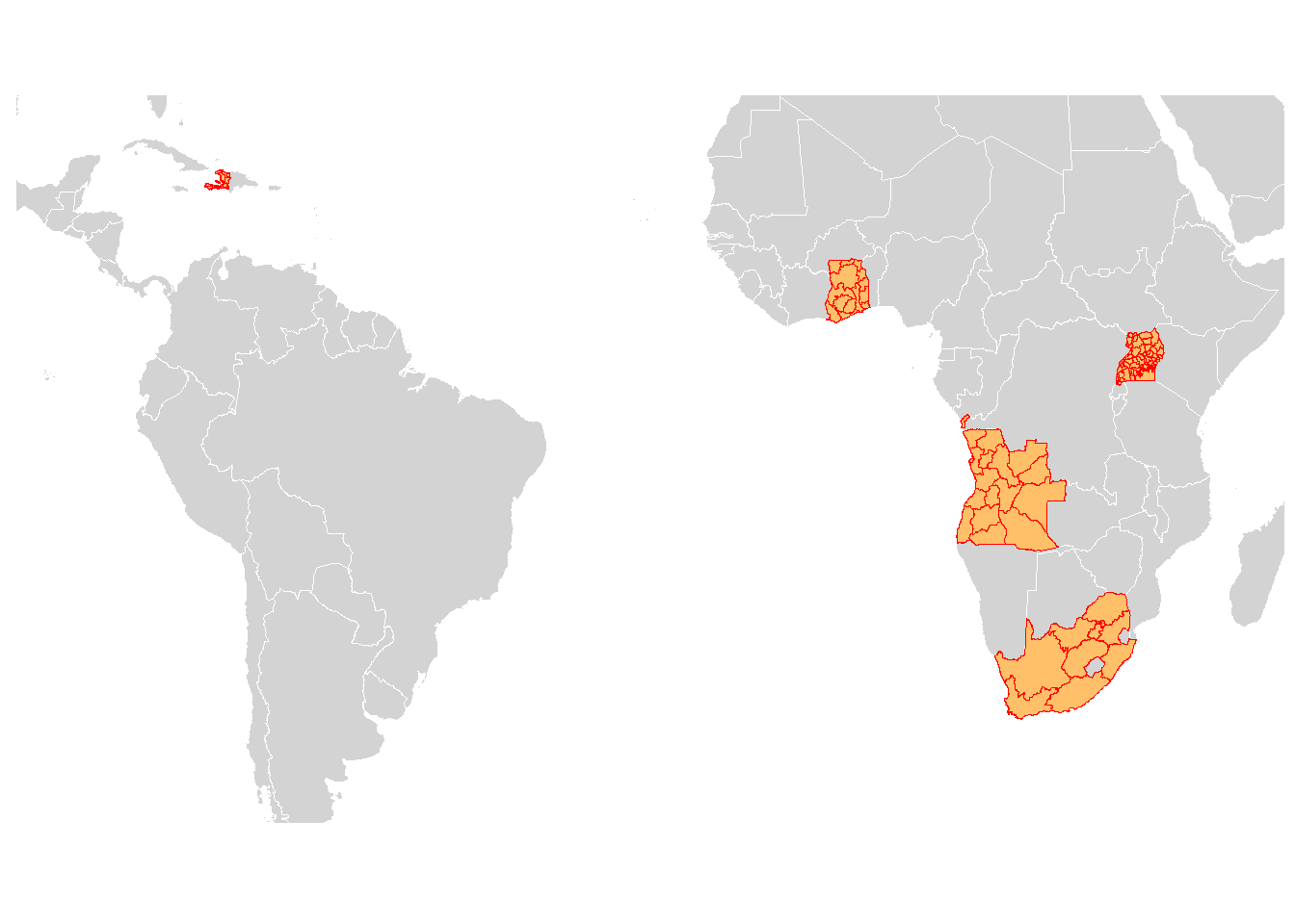
This post shows how to download and plot administrative areas from multiple countries on a world map. The main lesson is a subtle plotting bug: if region names are not unique across countries, ggplot2::geom_polygon() can draw strange connecting lines between unrelated areas.
Maintenance note: this example preserves the original sp/raster workflow. For new spatial work in R, sf, terra, and geodata are usually easier to maintain, but the polygon-grouping issue shown here is still relevant.
The basic map
(You may download the world map from GitHub)
suppressPackageStartupMessages({
library("data.table")
library("ggplot2")
library("rgdal")
library("raster")
library("rgeos")
library("here")
library("ggthemes")
})

# download data from GADM directly and row-bind the spatial polygons data frame
cnames <- c("Haiti", "Togo", "Uganda", "Ghana", "South Africa", "Angola")
download.GADM <- function(cname0) raster::getData("GADM", country = cname0, level = 1)
dt_geos <- raster::bind(lapply(cnames, download.GADM))
dt_geos <- sp::spTransform(dt_geos, CRS("+proj=robin")) # robin transformation
dt_geos_df <- broom::tidy(dt_geos, region = "GID_1")

  x_min <- min(dt_geos_df$long)*1.2
  x_max <- max(dt_geos_df$long)*1.2
  y_min <- min(dt_geos_df$lat)* 1.2
  y_max <- max(dt_geos_df$lat)* 1.2

  map_theme <- ggthemes::theme_map() +
    theme(legend.position = "bottom", legend.direction = "horizontal", legend.justification = c("center"))

  shp_world_robin <- readRDS(here::here("../Data/World.shp/sp.world.robin.rds")) # this has to be sourced locally
  ggplot() +
    geom_polygon(data = shp_world_robin, aes(x = long, y = lat, group = group), fill="lightgray",
                 colour = "white", size=0.05) +
    geom_polygon(data = dt_geos, aes(x = long, y = lat, group = group),
                 color = "red", size=0.05, fill="#ffc069")  +
    # if want to crop map:
    coord_fixed(xlim=c(x_min, x_max), ylim=c(y_min, y_max)) +
    map_theme +
    guides(fill = guide_legend(nrow = 1, title.position = "top"))
Mapping values by administrative area
Next, we add values to the map. These values can be merged directly to the spatial polygons object or to a data frame derived from it. Here I show the second approach: transform the sp object into a data frame first, then supply that data frame to ggplot2::geom_polygon().
In GADM admin 1 files, GID_1 is a unique identifier even after binding multiple countries. To make the bug visible, this example intentionally uses region names from NAME_1 as the region identifier. In my applied work, I sometimes had to merge estimates using those names.
# `region` will become the id/group used to identify each area
# Either broom::tidy or ggplot2::fortify can work:
# dt_geos_data <- broom::tidy(dt_geos, region = "NAME_1")
# dt_geos_data <- ggplot2::fortify(dt_geos, region = "NAME_1")

download.GADM.df <- function(cname0){
  dfsp <- raster::getData("GADM", country = cname0, level = 1) # download data from GADM
  dfsp <- sp::spTransform(dfsp, CRS("+proj=robin")) # robin transformation
  dfsf <- broom::tidy(dfsp, region = "NAME_1") # get df
  dfsf$country <- cname0 # add a country identifier
  return(setDT(dfsf))
}

dt_geos_data <- rbindlist(lapply(cnames, download.GADM.df))

# imagine we want to plot estimates, not only the map
dt_admin1 <- unique(setDT(dt_geos_data)[,.(country, id)])
set.seed(1234)
dt_admin1$value <- rgamma(nrow(dt_admin1), shape = 4, scale = 15) # some random values

setkey(dt_geos_data, country, id)
setkey(dt_admin1, country, id)
dt_geos_data_value <- dt_geos_data[dt_admin1]

legend_break <- c(0, 25, 50, 75,  100, 150, 200, 300, 500)
legend_label <- c("≤25", "25 to 50", "50 to 75", "75 to 100", "100 to 150","150 to 200","200 to 300",">300")
legend_color <- c("#80BD41", "#CFF4FF","#feec9f","#ffc069","#fa8c16","#d46b08","#ad4e00","#612500")
dt_geos_data_value$col <- cut(dt_geos_data_value$value, breaks = legend_break, labels = legend_label)
The bug: strange connecting lines
ggplot() +
  geom_polygon(data = shp_world_robin, aes(x = long, y = lat, group = group), fill="lightgray",
               colour = "white", size=0.05) +
  geom_polygon(data = dt_geos_data_value, aes(x = long, y = lat, group = group, fill= col),
               color = "red", size=0.05)  +
  coord_fixed(xlim=c(x_min, x_max), ylim=c(y_min, y_max)) + # crop map
  scale_fill_manual("Some random values for example", values = legend_color, drop = FALSE) +# Keep all legend item
  map_theme +
  guides(fill = guide_legend(nrow = 1, title.position = "top"))
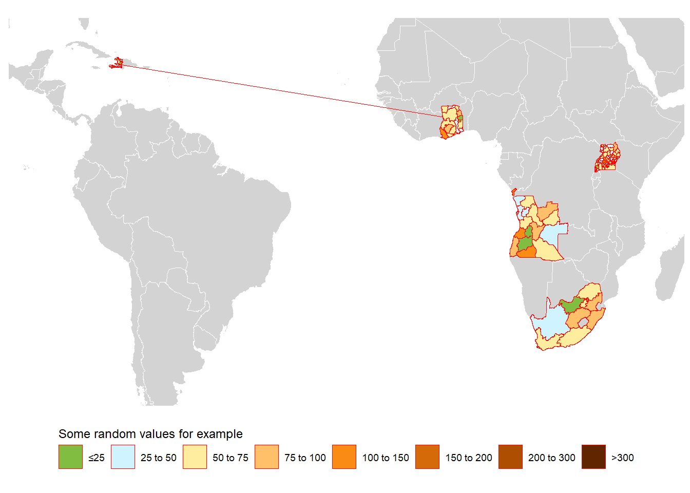
The problem is that some countries share admin 1 names from NAME_1 in the GADM file during the broom::tidy() or ggplot2::fortify() step.
In this example, Haiti and Togo share names such as Centre.1 and Centre.2 (see the table below).
The fix is to set group to an identifier that is unique across countries in ggplot2::geom_polygon():
dt_geos_data_value[, county_group := paste(country, group, sep = "_")]
unique(dt_geos_data_value[group %in% c("Centre.1"),.(country, id, group, county_group, value)])
## country id group county_group value
## 1: Haiti Centre Centre.1 Haiti_Centre.1 24.09058
## 2: Togo Centre Centre.1 Togo_Centre.1 54.32445ggplot() +
geom_polygon(data = shp_world_robin, aes(x = long, y = lat, group = group), fill="lightgray",
colour = "white", size=0.05) +
geom_polygon(data = dt_geos_data_value, aes(x = long, y = lat, group = county_group, fill= col),
# it's important to set `group = county_group` instead of `group = group`
color = "red", size=0.05) +
coord_fixed(xlim=c(x_min, x_max), ylim=c(y_min, y_max)) +
scale_fill_manual("Some random values for example", values = legend_color, drop = FALSE) +# Keep all legend item
map_theme +
guides(fill = guide_legend(nrow = 1, title.position = "top"))
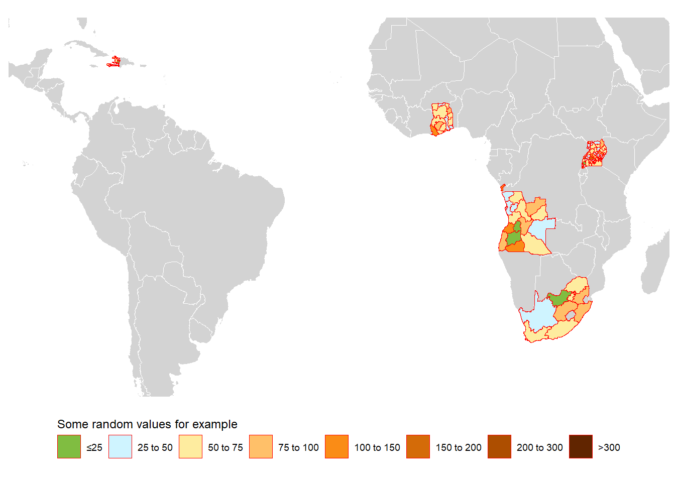
The key habit is to check whether the polygon grouping variable is unique after combining countries. If it is not, create a country-specific group ID before plotting.