Spatial data in R: Dividing raster layers into equal-area rings

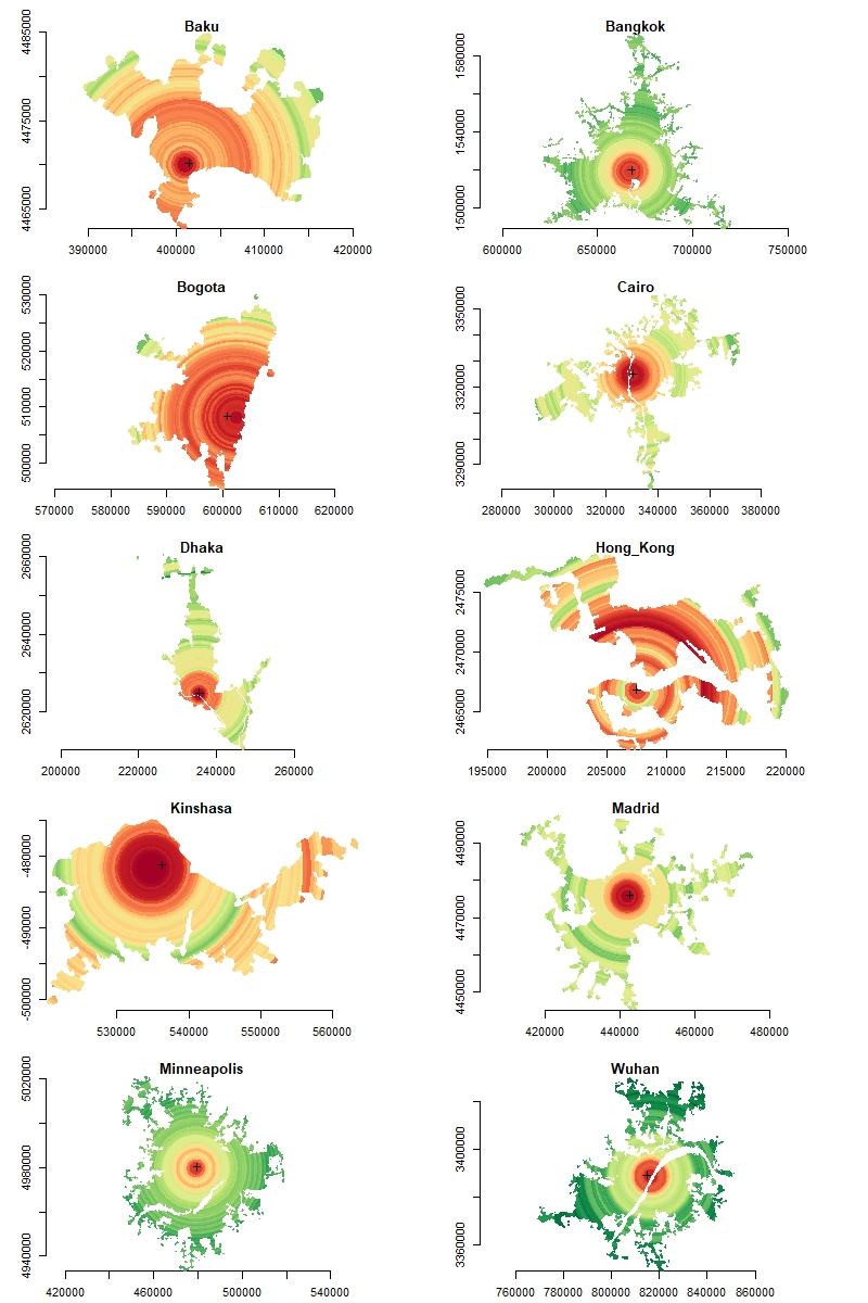
Saturation in ten cities with equal-area rings

• The 1000 rings have a minimum saturation of 30.5% and a maximum of 99.9%
  
• Same color scale for every map, with a boundary of [0.3, 1]
  
• Dark green corresponds to a ring saturation of 0.3, and dark red corresponds to 1

R Code for one city

• The setting of the code can loop around several different cities, here we only load one city.

list.of.packages <- c("raster", "rgdal", "Hmisc", "plyr", "RColorBrewer", "googledrive")
new.packages <- list.of.packages[!(list.of.packages %in% installed.packages()[,"Package"])]
if(length(new.packages)) install.packages(new.packages)

suppressPackageStartupMessages({
library('raster')   # obtain raster from GIS image file, and plot
library('rgdal')    # readOGR: read ArcGIS vector maps into Spatial objects
library('Hmisc')    # cut2: cut vector into equal-length
library('plyr')     # join
library('RColorBrewer') # for `brewer.pal` in ggplot2
library('knitr')    # kable
})
options(digits = 4)

• The local version:

# Where are all the data files located:
parent_dir <- c("D:/OneDrive - nyu.edu/NYU Marron/180716_Draw Circle/Data/")
# Get all the folder names (names of the cities) in the directory, used to scan all the cities
city_list <- list.files(parent_dir)

# If use Hong Kong as an example
  city1 <- city_list[6]
  newdir <- paste(parent_dir, city1, sep = "")
  image <- raster(paste(newdir, c("./city_urbFootprint_clp_t3.img"), sep = ""))
    
  # A point that shows the center of the city
  cbd <-  readOGR(dsn = newdir, layer = paste(city1, "_CBD_Project", sep=""))

## OGR data source with driver: ESRI Shapefile 
## Source: "D:\OneDrive - nyu.edu\NYU Marron\180716_Draw Circle\Data\Hong_Kong", layer: "Hong_Kong_CBD_Project"
## with 1 features
## It has 6 fields
## Integer64 fields read as strings:  Id

  cbdpoint <- SpatialPoints(cbd)

• In this blog data is downloaded from googledrive

city1 <-"Hong_Kong"
library(googledrive)
temp <- tempfile(fileext = ".zip")
dl <- drive_download(as_id("1z-aD2orN2k2BINkDD6whEhHFga_4HIu8"), path = temp, overwrite = TRUE)
out <- unzip(temp, exdir = tempdir())
image <- raster(out[1])
cbdpoint <- SpatialPoints(readOGR(dsn = paste(tempdir(),"\\Hong_Kong",sep = ""),
                                  layer = "Hong_Kong_CBD_Project"))

• Read raster as points: rasterToPoints

  # mydata_HK contains coordinate (x,y) and category (type)
  mydata_HK <- as.data.frame(rasterToPoints(image))
  names(mydata_HK) <- c("x", "y", "type")

• Divide points into ten equal-size rings
  
• Calculate distances using sp::spDistsN1

  # calculate distance to the cbd from every point
  pts <- as.matrix(mydata_HK[,1:2])
  mydata_HK$cbd_dist <- spDistsN1(pts, cbdpoint, longlat = F)
  
  # library('Hmisc') # cut2
  mydata_HK$ring <- as.numeric(cut2(mydata_HK$cbd_dist,g = 100)) # get 1:100
  mydata_HK$type <- as.factor(mydata_HK$type)
  mydata_HK$ring <- as.factor(mydata_HK$ring)

  # Function to get saturation, as the raster have 7 layers, 1 to 3 belong to built-up area
  get_sat <- function(x){
    x <- as.factor(x)
    # (1 + 2 + 3) / (1 + 2 + 3 + 4 + 5 + 6 + 7)
    sum(x==1|x==2|x==3)/length(x)
  }

  # get saturation by rings
  sat_output <- aggregate(mydata_HK$type, by = list(mydata_HK$ring), FUN = get_sat)
  names(sat_output) <- c("ring", "ring_saturation")
  # join back to mydata_HK2 so we can later plot by values of ring_saturation
  mydata_HK2 <- join(mydata_HK, sat_output, by = "ring")
  kable(head(mydata_HK2))  

x	y	type	cbd_dist	ring	ring_saturation
203936	2478244	3	11970	94	0.5318
203966	2478244	4	11961	94	0.5318
203996	2478244	4	11952	93	0.5721
204026	2478244	3	11944	93	0.5721
204056	2478244	4	11935	93	0.5721
204086	2478244	4	11926	93	0.5721

• Turn dataframe (mydata_HK2) into raster using rasterFromXYZ
  
• Numeric columns are automatically assigned as values in the raster, and if we plot it directly:

  r1 <- rasterFromXYZ(mydata_HK2)
  plot(r1)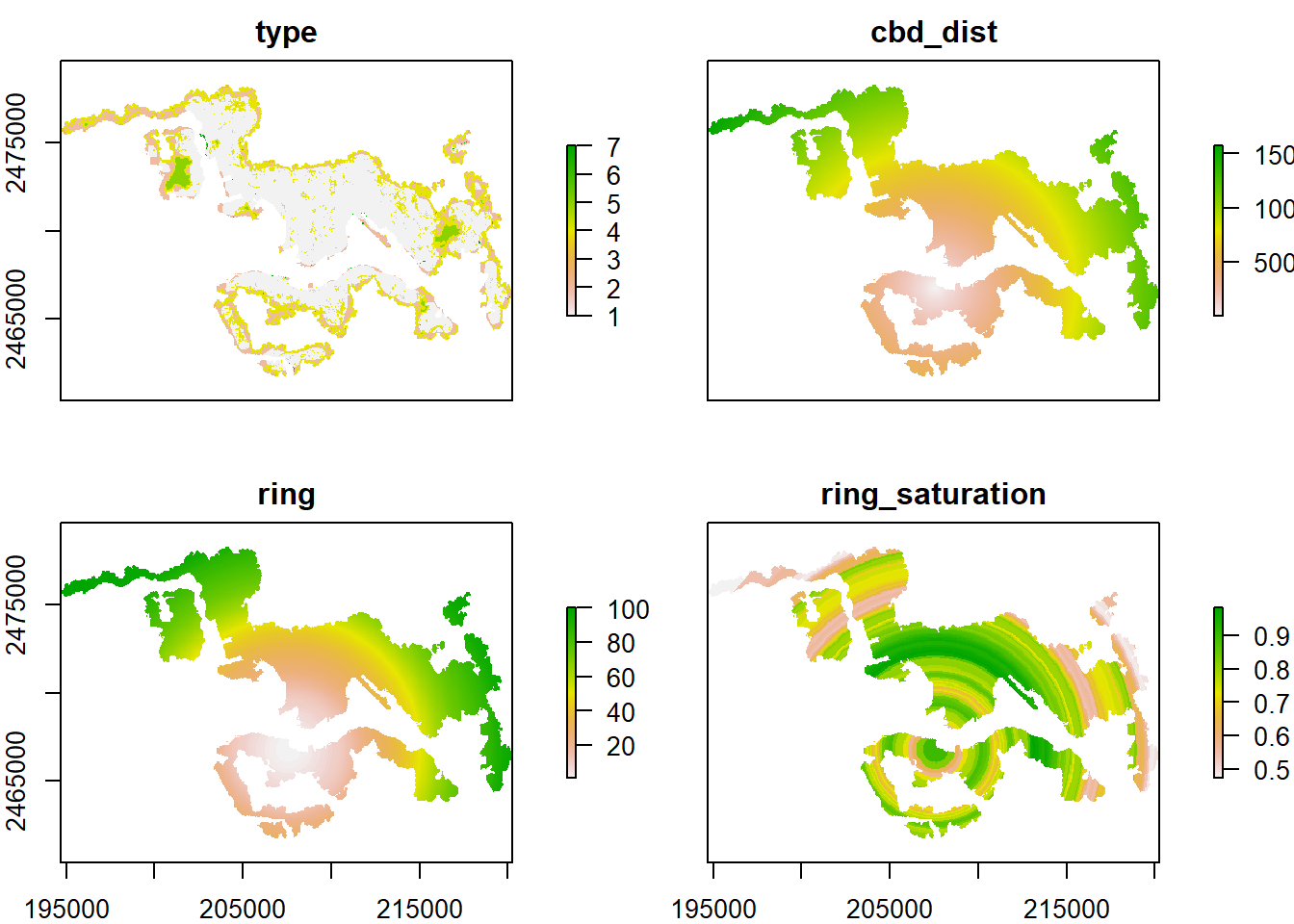

  # choose a color scale from `RColorBrewer`
  color_scale <- brewer.pal(n = 10, name = "RdYlGn")
  myPalette <- colorRampPalette(rev(color_scale)) # reverse the order so highly value ~ dark red
  # set col and breaks to align color scale across figures
  plot(r1$ring_saturation, col=myPalette(70), breaks = c(30:100)/100,
       legend=FALSE,  main = city1)
  plot(cbdpoint, add = TRUE, size = 3) # drawn on top of a map using `add = TRUE`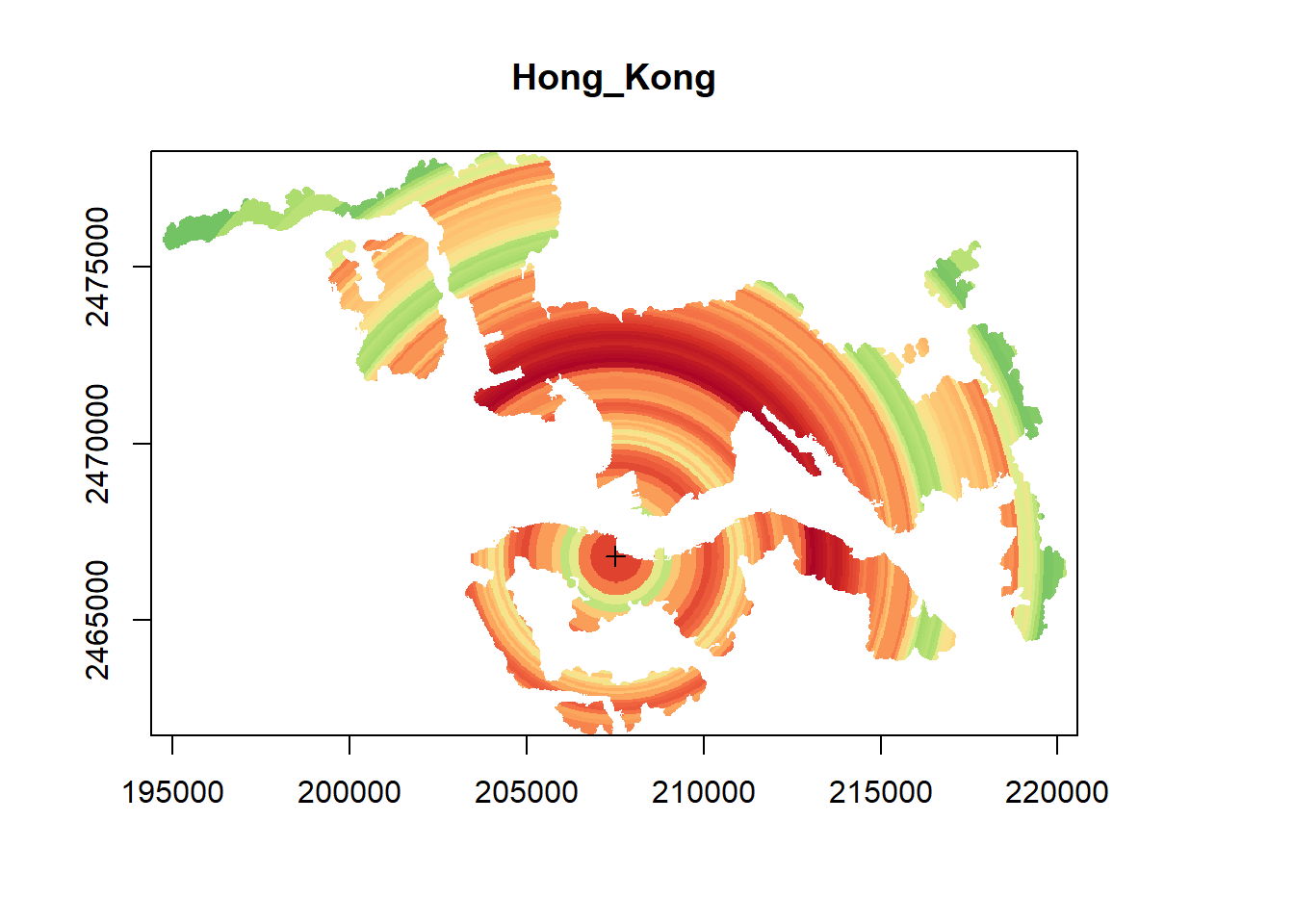

  # if need to output the raster
  # writeRaster(r1, paste(raster_dir, city1, sep = ""), format = "HFA", overwrite=TRUE)

  # To preview the color panel:
  # display.brewer.pal(n = 12, name = 'RdYlGn')

Results for the ring saturations

• I run the code using a loop for ten cities
  
• Ring saturation in the 10 cities has a minimum of 30.5% and a maximum of 99.9%:

#   Min. 1st Qu.  Median    Mean 3rd Qu.    Max. 
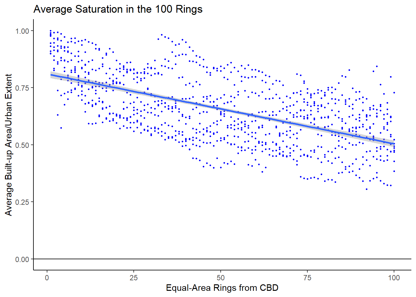
#  0.305   0.545   0.646   0.656   0.771   0.999 

Average saturation in each ring

• There is a clear declining trend in saturation as we move towards the boundary of the cities
  

Methodology

(Summarized by Alejandro Blei, my colleague)
1. Take the file: city_urbFootprint_clp_t3.img. This file is made up of many pixels. Pixels with values 1-3 = built up, pixels with values 4-6 = open space, and pixels with value 7 = water. In other words, 1 - 3 = built up, and 4 - 7 = not built.
2. Convert the pixels to points. This operation preserves the value associated with the pixel.
3. Calculate the distance from each point to the CBD.
4. Create 10 groups from these pixels, where each group has the same area. These groups radiate outward from the CBD. Since each pixel has the same size, all we need are ten groups with the same number of pixels, where the pixels in one group are closer to the CBD than the pixels in the next group.
5. Once we have the groups, we can calculate the saturation value in each group. Saturation is Built Up / (Built Up - Open Space), in other words, saturation is Pixels (1 + 2 + 3) / (1 + 2 + 3 + 4 + 5 + 6 + 7). Each of the ten groups now has a saturation value associated with it.

Original Code

• Local version, loop over ten cities

# Fragmentation: Saturation  (Built-up Area/Urban Extent) in each ring
# how about 100 rings

# install.packages('raster')
library('raster')   # obtain raster from GIS image file, and plot
library('rgdal')    # readOGR: read ArcGIS vector maps into Spatial objects
library('Hmisc')    # cut2
library('plyr')     # join
library('RColorBrewer') # for `brewer.pal` in ggplot2
library('knitr')    # kable
options(digits = 4)

# get saturation
get_sat <- function(x){
  x <- as.factor(x)
  # (1 + 2 + 3) / (1 + 2 + 3 + 4 + 5 + 6 + 7)
  sum(x==1|x==2|x==3)/length(x)
}

parent_dir <- c("D:/OneDrive - nyu.edu/NYU Marron/180716_Draw Circle/Data/")
# Get all the folder names (names of the cities) in the directory
city_list <- list.files(parent_dir)

sat_out <- data.frame()
par(mar = c(1,2,1,0), bty="n") # c(bottom, left, top, right)
layout(matrix(c(1:10),ncol=2, byrow = T))
# length(city_list)
for (i in 1:10){
  city1 <- city_list[i]
  newdir <- paste(parent_dir, city1, sep = "")
  image <- raster(paste(newdir, c("./city_urbFootprint_clp_t3.img"), sep = ""))
  # mydata: df that contains coordinate and category
  mydata <- as.data.frame(rasterToPoints(image))
  names(mydata) <- c("x", "y", "type")
  pts <- as.matrix(mydata[,1:2])
  
  # cbd
  cbd <-  readOGR(dsn = newdir, layer = paste(city1, "_CBD_Project", sep=""))
  cbdpoint <- SpatialPoints(cbd)

  # distance to the cbd
  mydata$cbd_dist <- spDistsN1(pts, cbdpoint, longlat = F)
  # library('Hmisc') # cut2
  mydata$ring <- as.numeric(cut2(mydata$cbd_dist,g = 100))
  mydata$type <- as.factor(mydata$type)
  mydata$ring <- as.factor(mydata$ring)

  
  sat_output <- aggregate(mydata$type, by = list(mydata$ring), FUN = get_sat)
  sat_output$City <- city1
  sat_output$City_Saturation <- get_sat(mydata$type)
  names(sat_output) <- c("ring", "ring_saturation","city", "city_saturation")
  sat_out <- rbind(sat_out, sat_output)
  

  # draw the figure ---------------------------------------------------------
  
  mydata2 <- join(mydata, sat_output, by = "ring")
  r1 <- rasterFromXYZ(mydata2)
  # writeRaster(r1, paste(raster_dir, city1, sep = ""), format = "HFA", overwrite=TRUE)

  # To preview the color panel:
  # display.brewer.pal(n = 12, name = 'RdYlGn')
  color_scale <- brewer.pal(n = 10, name = "RdYlGn")
  myPalette <- colorRampPalette(rev(color_scale))

  plot(r1$ring_saturation, col=myPalette(70), breaks = c(30:100)/100,
       legend=FALSE,  main = city1)
  plot(cbdpoint, add = TRUE, size = 3) # drawn on top of a map using `add = TRUE`

}


# Some visulization options -----------------------------------------------------------
id <- "1DNyQLX0apRVWmRC1xKhpqZLE6SLcQF5p" # google file ID
sat <- read.csv(sprintf("https://docs.google.com/uc?id=%s&export=download", id))
sat$idx <- rep(c(1:100),10)

# linear regression smoothing
ggplot(sat, aes(x=idx, y=ring_saturation)) +
  geom_point(size = 0.5, color = 'blue') +  
  geom_smooth(method = 'lm')+
  theme_classic() + 
  geom_hline(yintercept = 0) +
  scale_y_continuous(limits = c(0,1)) +
  labs(x = "Equal-Area Rings from CBD", y = "Average Built-up Area/Urban Extent") +
  ggtitle("Average Saturation in the 100 Rings")

## some other options
# one plot for each city
par(mar = rep(2,4), bty="n")
layout(matrix(c(1:10),ncol=2, byrow = T))
for (i in 1:10){
  sat_sub <- subset(sat, city == city_list[i])
  plot(x = sat_sub$idx, y = sat_sub$ring_saturation, type = "l",
       xlab=c("Ring from CBD"), ylab =c("Built-up Area/Urban Extent"),
       main = city_list[i])
}

# a barchart for each ring?
sat$weight_blank <- 1
source("D:/OneDrive - nyu.edu/NYU Marron/R/Get Weighted SE and CI.R")
Mean_byGroup <- get_WM_and_CI2(sat, "idx", "ring_saturation", "weight_blank") 
bar_width <- 0.8
ggplot(Mean_byGroup, aes(x=idx, y=wm, 
                         ymin=CI_low, ymax=CI_high)) +
  geom_bar(stat='identity', position = position_dodge(), width = bar_width, alpha=0.8)+
  geom_errorbar (width=bar_width-0.1, lwd=1, position=position_dodge(bar_width))+
  labs(x = "Ten Rings from CBD", y = "Average Built-up Area/Urban Extent") +
  ggtitle("Average Saturation in Each Ring")+
  theme_classic()  +  
  geom_hline(yintercept = 0)

# scatterplot all the points for ten cities 
ggplot(sat, aes(x=idx, y=ring_saturation, color = city)) +
  geom_point(size = 1) 
  labs(x = "Ten Rings from CBD", y = "Built-up Area/Urban Extent") +
  ggtitle("Saturation in Each Ring of Ten Cities")+
  theme_classic()