Using SHAPforxgboost with LightGBM • SHAPforxgboost

Introduction

This vignette shows how to use SHAPforxgboost for interpretation of models trained with LightGBM, a hightly efficient gradient boosting implementation (Ke et al. 2017).

library("ggplot2")
library("SHAPforxgboost")
library("lightgbm")

set.seed(9375)

Training the model

Let’s train a small model to predict the first column in the iris data set, namely Sepal.Length.

head(iris)
#>   Sepal.Length Sepal.Width Petal.Length Petal.Width Species
#> 1          5.1         3.5          1.4         0.2  setosa
#> 2          4.9         3.0          1.4         0.2  setosa
#> 3          4.7         3.2          1.3         0.2  setosa
#> 4          4.6         3.1          1.5         0.2  setosa
#> 5          5.0         3.6          1.4         0.2  setosa
#> 6          5.4         3.9          1.7         0.4  setosa

X <- data.matrix(iris[, -1])

fit <- lgb.train(
  params = list(objective = "regression"),
  data = lgb.Dataset(X, label = iris[[1]]),
  nrounds = 50,
  verbose = -2
)

SHAP analysis

Now, we can prepare the SHAP values and analyze the results. All this in just very few lines of code!

# Crunch SHAP values
shap <- shap.prep(fit, X_train = X)

# SHAP importance plot
shap.plot.summary(shap)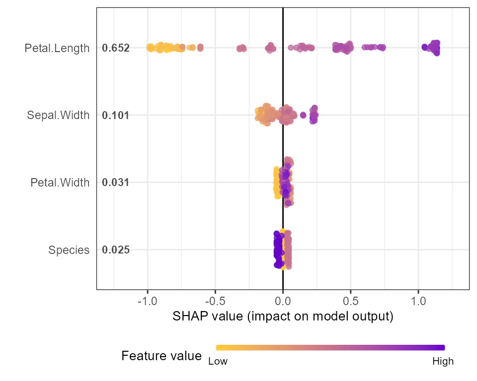


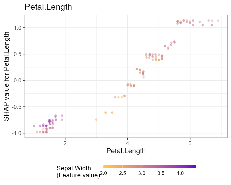
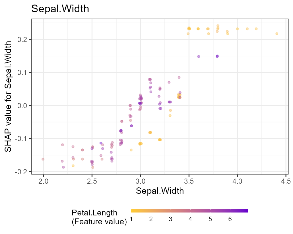
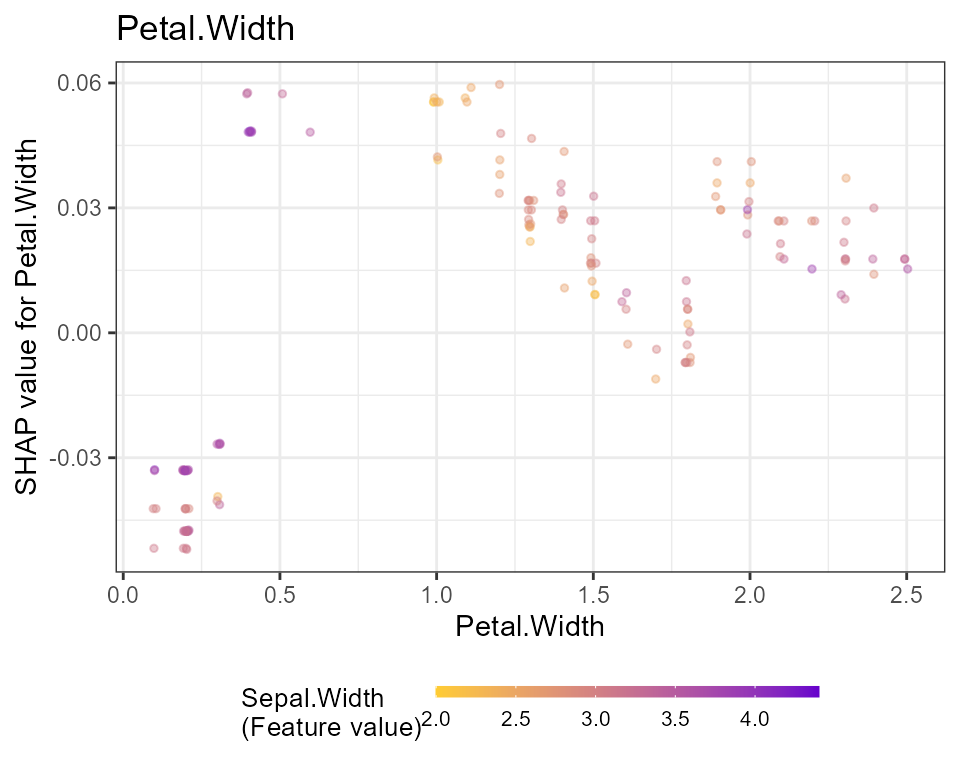
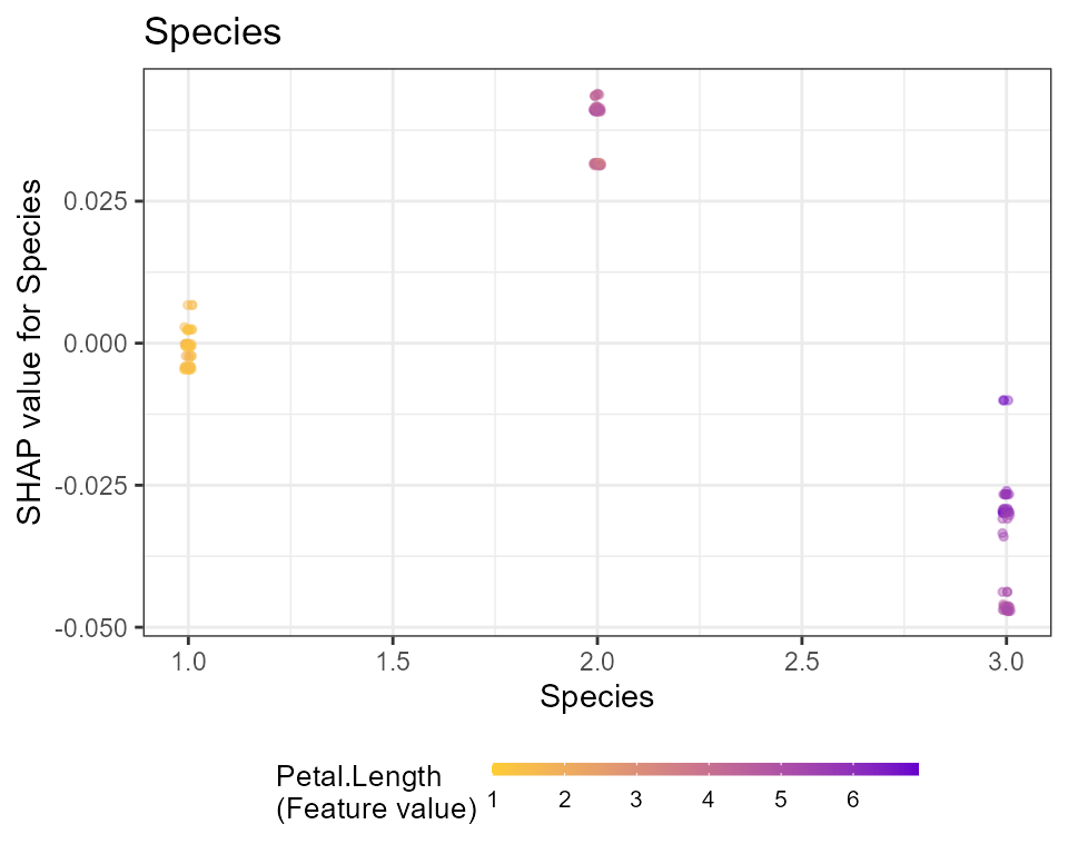
# Dependence plots in decreasing order of importance
for (x in shap.importance(shap, names_only = TRUE)) {
  p <- shap.plot.dependence(
    shap, 
    x = x, 
    color_feature = "auto", 
    smooth = FALSE, 
    jitter_width = 0.01, 
    alpha = 0.4
    ) +
  ggtitle(x)
  print(p)
}

Note: print is required only in the context of using ggplot in rmarkdown and for loop.

References

Ke, Guolin, Qi Meng, Thomas Finely, Taifeng Wang, Wei Chen, Weidong Ma, Qiwei Ye, and Tie-Yan Liu. 2017. “LightGBM: A Highly Efficient Gradient Boosting Decision Tree.” In Advances in Neural Information Processing Systems 30 (NIP 2017).