A wrapped function to make summary plot from model object and predictors

shap.plot.summary.wrap1 wraps up function shap.prep and shap.plot.summary

shap.plot.summary.wrap1(model, X, top_n, dilute = FALSE)

Arguments

model	the model
X	the dataset of predictors used for calculating SHAP
top_n	how many predictors you want to show in the plot (ranked)
dilute	being numeric or logical (TRUE/FALSE), it aims to help make the test plot for large amount of data faster. If dilute = 5 will plot 1/5 of the data. If dilute = TRUE or a number, will plot at most half points per feature, so the plotting won't be too slow. If you put dilute too high, at least 10 points per feature would be kept. If the dataset is too small after dilution, will just plot all the data

Examples

data("iris")
X1 = as.matrix(iris[,-5])
mod1 = xgboost::xgboost(
  data = X1, label = iris$Species, gamma = 0, eta = 1,
  lambda = 0, nrounds = 1, verbose = FALSE)

# shap.values(model, X_dataset) returns the SHAP
# data matrix and ranked features by mean|SHAP|
shap_values <- shap.values(xgb_model = mod1, X_train = X1)
shap_values$mean_shap_score
#> Petal.Length  Petal.Width Sepal.Length  Sepal.Width 
#>   0.62935975   0.21664035   0.02910357   0.00000000 
shap_values_iris <- shap_values$shap_score

# shap.prep() returns the long-format SHAP data from either model or
shap_long_iris <- shap.prep(xgb_model = mod1, X_train = X1)
# is the same as: using given shap_contrib
shap_long_iris <- shap.prep(shap_contrib = shap_values_iris, X_train = X1)

# **SHAP summary plot**
shap.plot.summary(shap_long_iris, scientific = TRUE)
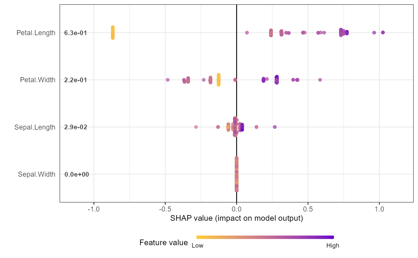shap.plot.summary(shap_long_iris, x_bound  = 1.5, dilute = 10)

# Alternatives options to make the same plot:
# option 1: from the xgboost model
shap.plot.summary.wrap1(mod1, X = as.matrix(iris[,-5]), top_n = 3)

# option 2: supply a self-made SHAP values dataset
# (e.g. sometimes as output from cross-validation)
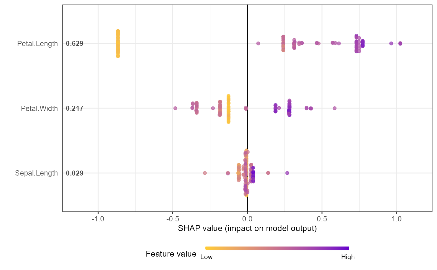
shap.plot.summary.wrap2(shap_score = shap_values_iris, X = X1, top_n = 3)